Diffusion LLMs from the Ground Up: Theory, Math, and Why They Work
Diffusion LLMs Part 1: Understanding how diffusion language models work from first principles, the math behind masked diffusion, and why they represent a fundamentally different approach to text generation.
Intro
Every production LLM today generates text the same way, i.e., one token at a time, left to right. GPT-4, Claude, Gemini, DeepSeek, LLaMA. All of them use autoregressive (AR) generation, where each token depends on every token before it.
This creates two structural problems. First, it's slow in a way that better hardware can't fully fix. Second, it creates blind spots in reasoning that no amount of training data can patch.
Diffusion language models (dLLMs) take a fundamentally different approach. Instead of generating tokens sequentially, they start with a fully masked sequence and iteratively reveal all tokens in parallel, refining the output over multiple steps.
This gives a generation paradigm that's compute-efficient, bidirectional, and capable of things autoregressive models structurally can't do.
This article builds a complete understanding of how dLLMs work, from first principles to the math. By the end, you should be able to read any dLLM paper fluently, understand every component of the architecture, and reason about why this approach works.
Let's begin.
The sequential bottleneck in autoregressive generation
Autoregressive models factorize the probability of a text sequence as a product of conditional probabilities:
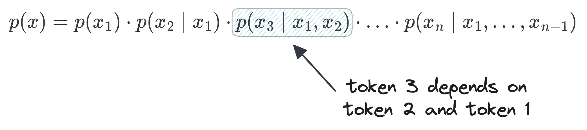
Each factor $p(x_i|x_1,\ldots,x_{i-1})$ represents the probability of the next token given everything before it. This is called the chain rule of probability, and it's mathematically exact.
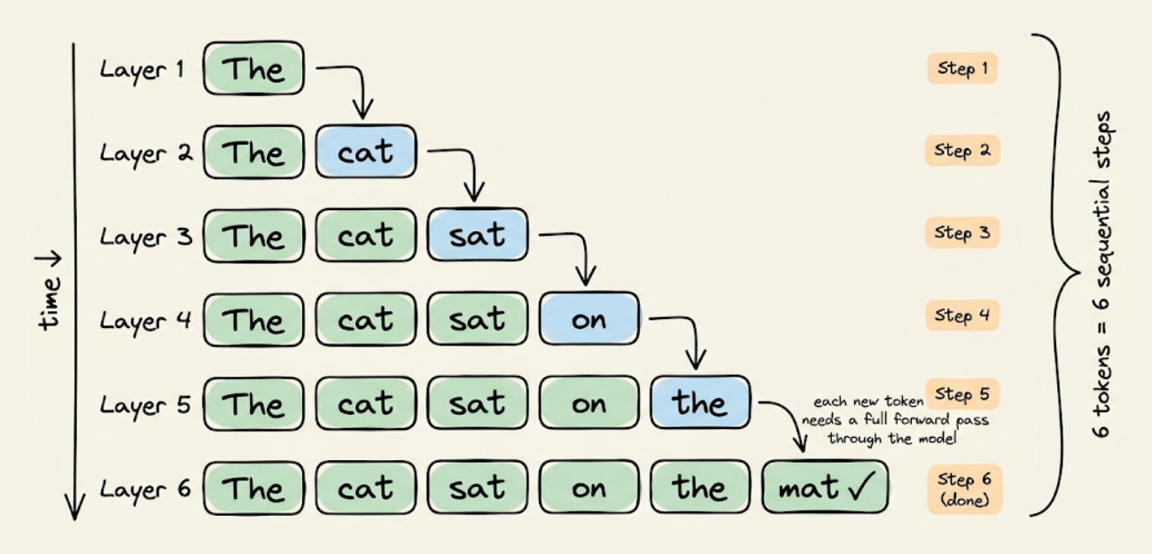
The key point here is that each factor requires its own forward pass through the model.
Each of these factors in the above mathematical formulation requires loading the full model weights through GPU memory to produce a single token.
To understand better, consider what happens during autoregressive decoding at the hardware level.
A 7B parameter model stored in FP16 precision occupies roughly 14GB of GPU memory.
To generate a single token, the GPU needs to read those 14GB of weights from its high-bandwidth memory (HBM) into its compute cores, perform the matrix multiplications and attention computations, and produce one output token. Then, for the next token, it reads all 14GB again.
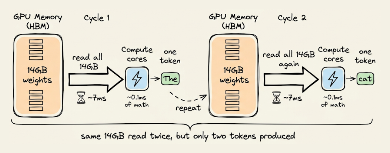
The reading part is the bottleneck. An A100 GPU can read data from HBM at about 2 TB/s. Reading 14GB at that speed takes roughly 7 milliseconds. The actual math (all the matrix multiplies, the attention scores, the MLP layers) may be takes about 0.1 milliseconds.
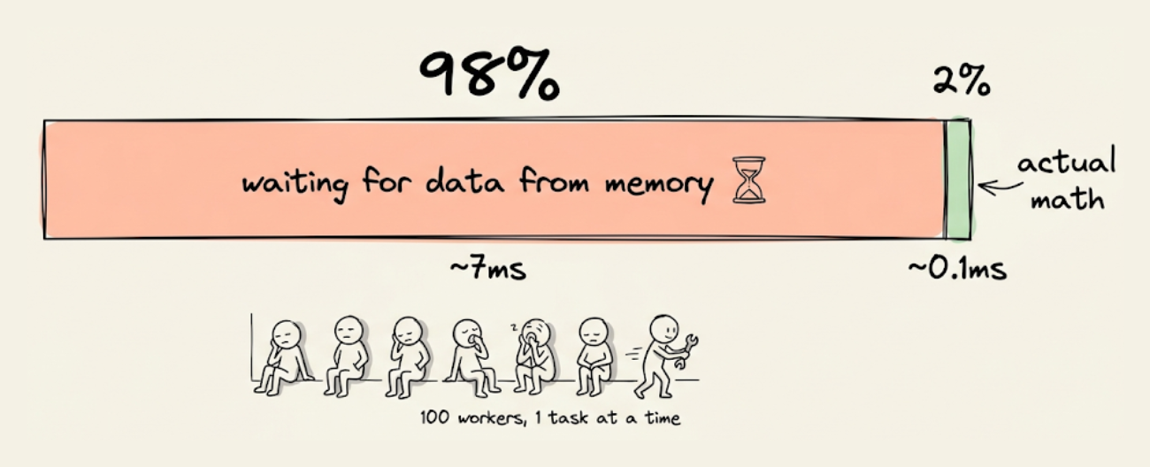
So the GPU spends 7ms waiting for data that it then uses for a computation that takes 0.1ms. This means roughly 98% of the time spent on data transfer and only 2% on actual math.
A useful way to quantify this imbalance is arithmetic intensity, which is the ratio of compute operations (FLOPs) to bytes of data moved.
During Autoregressive decoding, this ratio is roughly 1 FLOP per byte. Modern GPUs like the A100 are designed for workloads with 100+ FLOPs per byte.
To put that in perspective, the GPU's compute cores are capable of performing 100 operations for every byte of data that arrives from memory.
But autoregressive decoding only needs 1 operation per byte. So the compute cores finish their work almost instantly and then sit waiting for the next chunk of data to arrive.
It's like having a team of 100 workers but only ever giving them 1 task at a time. They're not overloaded with work; they're waiting on the supply line.
The GPU is being used at roughly 1% of its computational capacity, not because the model is small, but because the memory system can't deliver data fast enough to keep the cores busy.
This is what it means for autoregressive decoding to be memory-bandwidth bound. The limiting factor isn't the GPU's ability to do math, it's how fast data can be shuttled from memory to the compute cores.
Buying a GPU with 2x more FLOPs doesn't help much if the memory bandwidth only improves by 1.3x. The gap between compute capability and memory bandwidth has been widening with every GPU generation, which means the Autoregressive bottleneck gets proportionally worse over time, not better.
The second structural problem is directional.
Autoregressive models only ever see left-to-right context during generation. This creates what's known as the reversal curse, where a model trained on documents containing "Tom Cruise's mother is Mary Lee Pfeiffer" will be significantly worse at answering "Who is Mary Lee Pfeiffer's son?" than "Who is Tom Cruise's mother?"
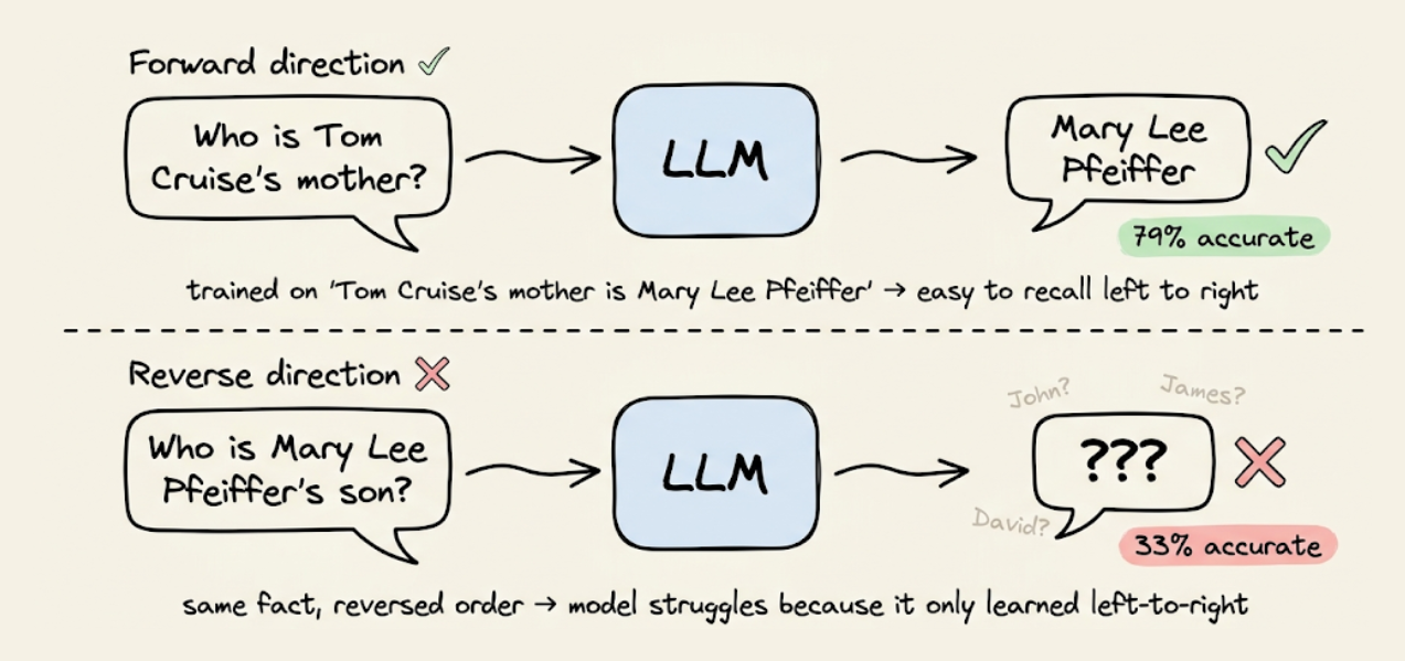
The original paper testing this on GPT-4 found 79% accuracy on the forward direction versus 33% on the reverse for 1,000 celebrity-parent pairs.
The asymmetry is caused by the autoregressive training objective. The model learns $p(\text{mother} | \text{Tom Cruise})$ but not $p(\text{Tom Cruise} | \text{mother's name})$ unless that ordering also appears in the training data.
The reversal curse is strongest for rare or obscure facts that predominantly appear in one ordering in the training data. For well-known facts like "Paris is the capital of France," the relationship appears in so many different orderings across a large training corpus that frontier models handle the reversal fine. The curse also doesn't apply to in-context reasoning: if you provide "A is B" in the prompt, autoregressive models can deduce "B is A" without issue.
The limitation is about what the model learns during training from left-to-right factorization, not about its reasoning ability at inference time.
Still, for long-tail knowledge (which is most knowledge), the asymmetry is measurable and significant, and it's a direct consequence of unidirectional training.
These two bottlenecks (sequential generation that underutilizes hardware, and unidirectional context that creates reasoning blind spots) are structural properties of the autoregressive factorization itself. They motivate the search for a fundamentally different generation paradigm.
How diffusion works in images?
Before we look at diffusion for text, it helps to understand how diffusion works in the domain where it first succeeded, i.e., images.
The core idea is surprisingly simple, and understanding it will make the text case (and the problems it introduces) much clearer.
The forward process: systematically destroying data
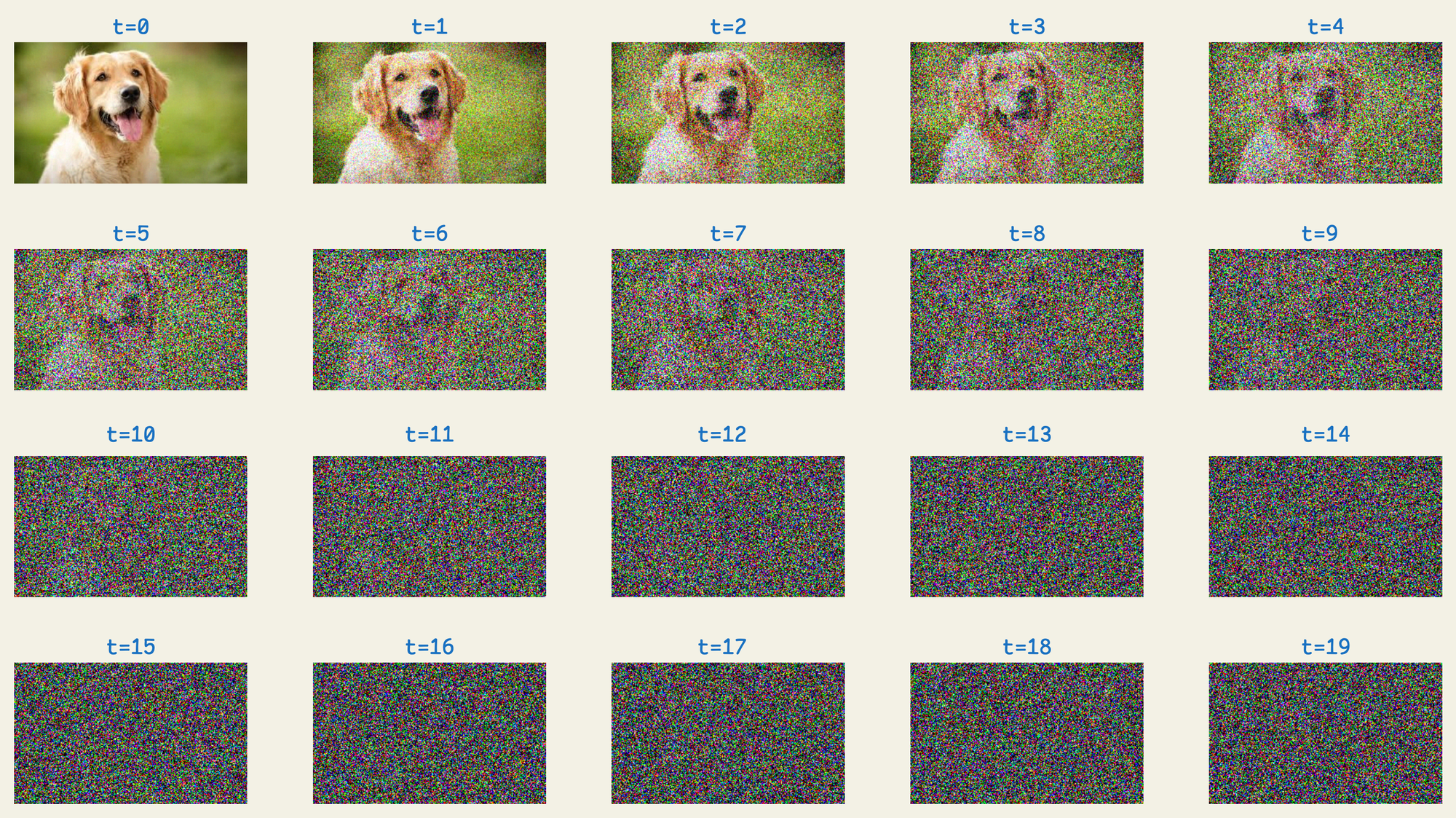
A diffusion model starts with a clean image and progressively corrupts it by adding Gaussian noise over many timesteps. At each step, a small amount of random noise is added to every pixel value. After enough steps, the image becomes pure noise, indistinguishable from random static.
Formally, given clean data $x_0$ (the original image), the forward process at timestep $t$ produces:
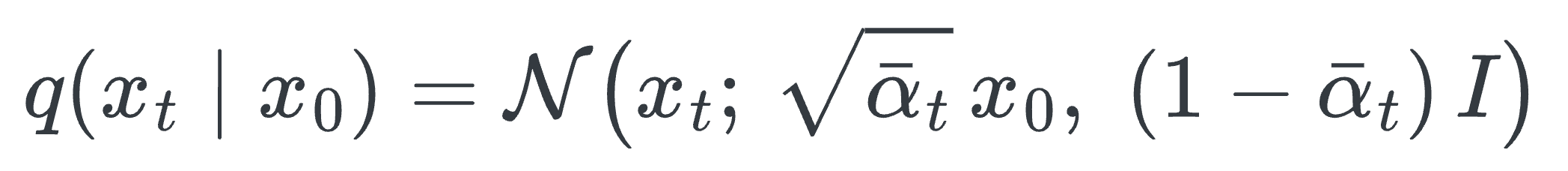
There are several components here, so let's unpack each one.