Gaussian Mixture Models (GMMs)
Gaussian Mixture Models: A more robust alternative to KMeans.
Introduction
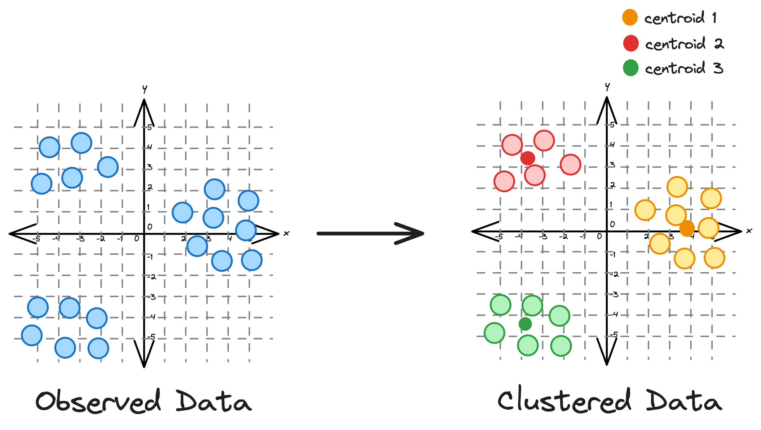
KMeans is an unsupervised clustering algorithm that groups data based on distances. It is widely recognized for its simplicity and effectiveness as a clustering algorithm.
Essentially, the core idea is to partition a dataset into distinct clusters, with each point belonging to the cluster whose centroid is closest to it.
While its simplicity often makes it the most preferred clustering algorithm, KMeans has many limitations that hinder its effectiveness in many scenarios.
The shortcomings of KMeans Clustering
KMeans comes with its own set of limitations that can restrict its performance in certain situations.
#1) KMeans does not account for cluster variance
One of the primary limitations is its assumption of spherical clusters.
One intuitive and graphical way to understand the KMeans algorithm is to place a circle at the center of each cluster, which encloses the points.
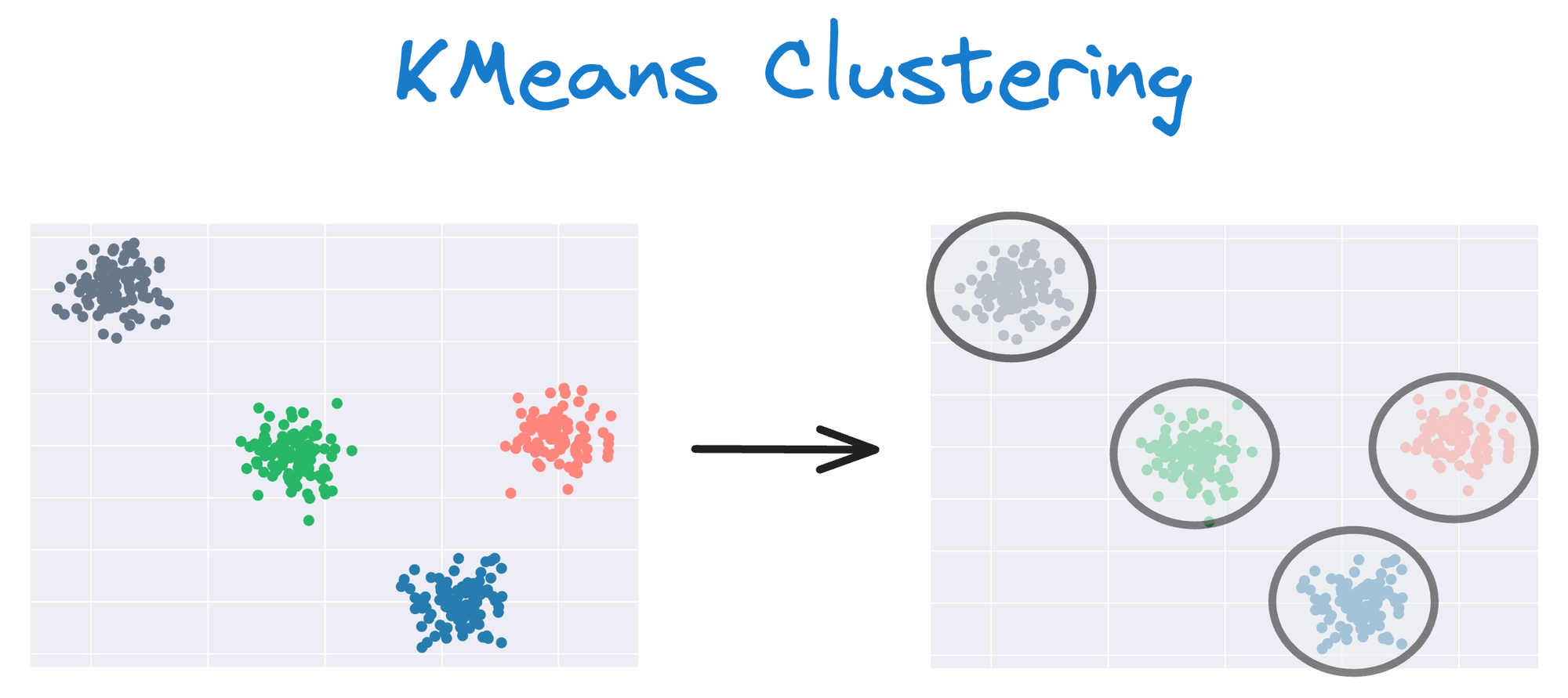
As KMeans is all about placing circles, its results aren’t ideal when the dataset has irregular shapes or varying sizes, as shown below:
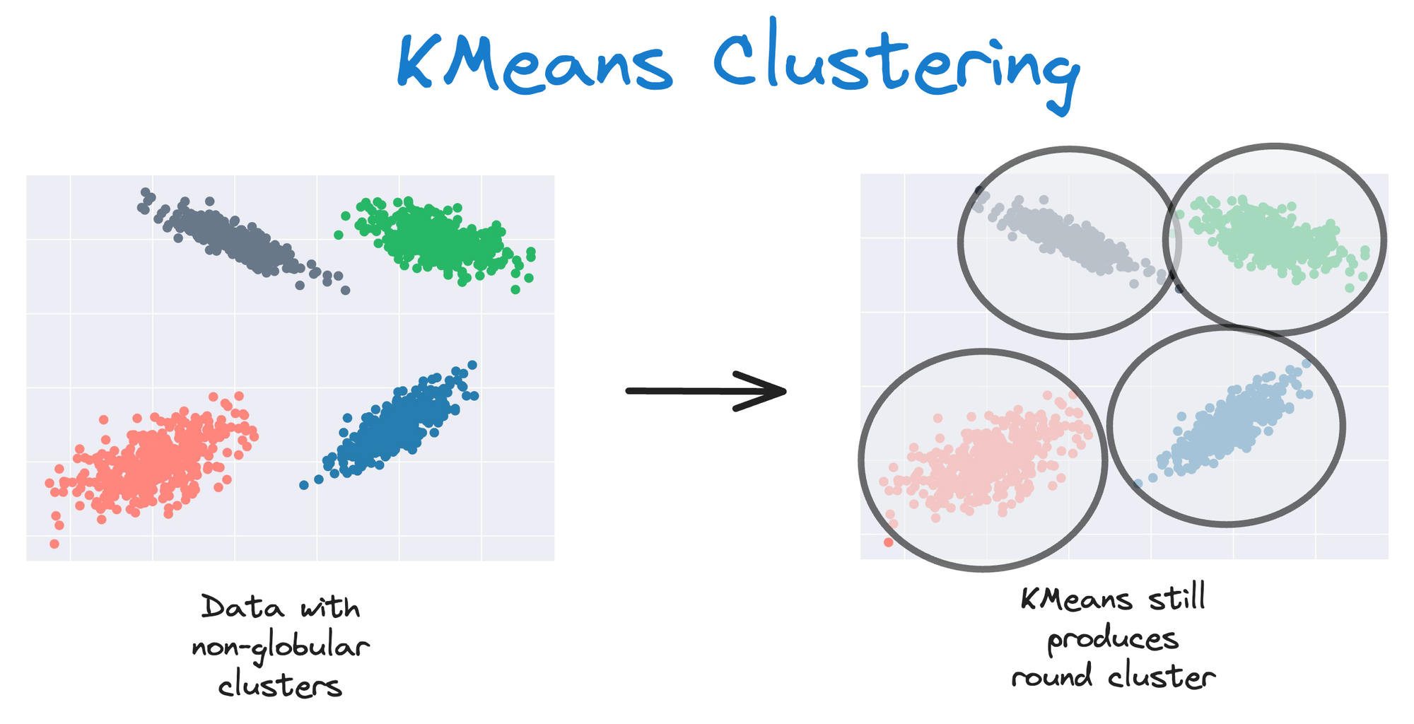
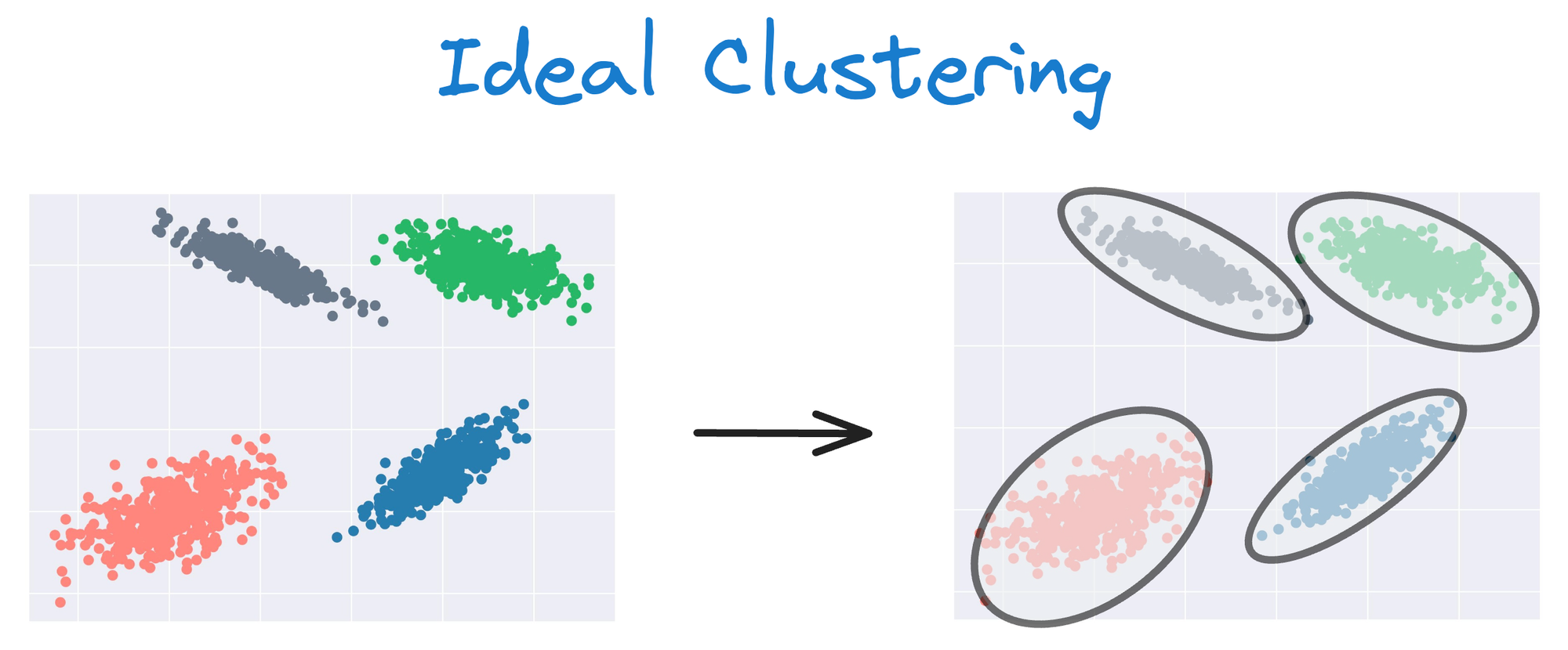
Instead, an ideal clustering should cluster the data as follows:
This rigidity of KMeans to only cluster globular clusters often leads to misclassification and suboptimal cluster assignments.
#2) KMeans only relies on distance
This limitation is somewhat connected to the one we discussed above.
Imagine we have the following dataset:
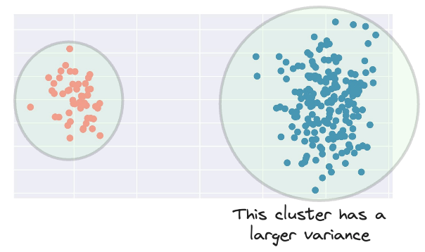
Clearly, the blue cluster has a larger spread.
Therefore, ideally, its influence should be larger as well.
However, when assigning a new data point to a cluster, KMeans only considers the distance to the centroid.
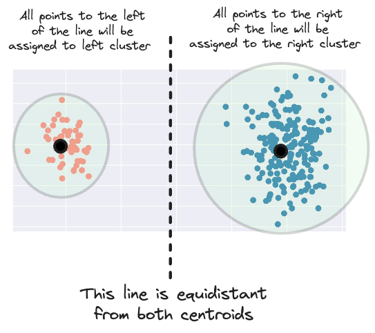
This means that it creates a margin for assigning a new data point to a cluster that is equidistant from both centroids.
But considering the area of influence of the right cluster, having this margin more to the left makes more sense.
#3) KMeans does not output probabilities
KMeans clustering performs hard assignments.
In simple words, this means that a specific data point can belong to only one cluster.

Thus, it does not provide probabilistic estimates of a given data point belonging to each possible cluster.
Although this might be a problem per se, it limits its usefulness in uncertainty estimation and downstream applications that require a probabilistic interpretation.
These limitations often make KMeans a non-ideal choice for clustering.
Therefore, learning about other better algorithms that we can use to address these limitations is extremely important.
Therefore, in this article, we will learn about Gaussian mixture models.
More specifically, we shall cover:
- Shortcomings of KMeans (already covered above)
- What is the motivation behind GMMs?
- How do GMMs work?
- The intuition behind GMMs.
- Plotting some dummy multivariate Gaussian distributions to better understand GMMs.
- The entire mathematical formulation of GMMs.
- How to use Expectation-Maximization to model data using GMMs?
- Coding a GMM from scratch (without sklearn).
- Comparing results of GMMs with KMeans.
- How to determine the optimal number of clusters for GMMs?
- Some practical use cases of GMMs.
- Takeaways.
Let's begin!
Gaussian Mixture Models
As the name suggests, a Gaussian mixture model clusters a dataset that has a mixture of multiple Gaussian distributions.
They can be thought of as a generalized twin of KMeans.
Simply put, in 2 dimensions, while KMeans only create circular clusters, gaussian mixture models can create oval-shaped clusters.
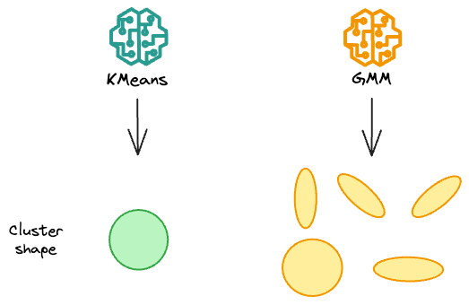
But how do they do that?
Let's understand in more detail.