Why R-squared is a Flawed Regression Metric?
The lesser-known limitations of the R-squared metric.
Introduction
Once you have trained any regression model, the next step is determining how well the model is doing.
Thus, it’s obvious to use a handful of performance metrics to evaluate the performance of linear regression, such as:
- Mean Squared Error – Well, technically, this is a loss function. But MSE is often used to evaluate a model as well.
- Visual inspection by plotting the regression line. Yet, this is impossible when you fit a high-dimensional dataset.
- R-Squared – also called the coefficient of determination.
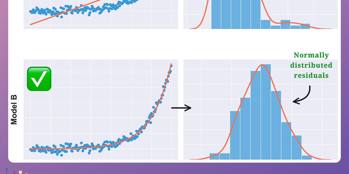
- Residual analysis (for linear regression) – involves examining the distribution of residuals to check for normality, as demonstrated in one of the earlier posts of Daily Dose of Data Science.
- F-statistic – Used to measure how much we are doing better than predicting the mean at a specific model inaccuracy.
We use them because evaluating the performance is crucial to ensure the model’s reliability and usefulness in a downstream application.
Also, performance quantification helps us make many informed decisions, such as:
- Do we need more feature engineering?
- Are we overfitting/underfitting the data, etc.?
The highlight of this article is the R-squared ($R^{2}$).
The $R^{2}$ metric is a popular choice among data scientists and machine learning engineers.
However, unknown to many, $R^{2}$ is possibly one of the most flawed evaluation metrics you could ever use to evaluate regression models.
Thus, in this blog, we’ll understand what is the $R^{2}$ metric, what it explains, and how to interpret it.
Further, we’ll examine why using the $R^{2}$ metric is not wise for evaluating regression models.
Let’s begin!
What is R-squared (R²)?
Before exploring the limitations of $R^{2}$, it is essential to understand its purpose and significance in linear regression analysis.
Essentially, when working with, say, a linear regression model, you intend to define a linear relationship between the independent variables (predictors) and the dependent variable (outcome).
$$ \Large \hat y = w_{1}*x_{1} + w_{2}*x_{2} + \dots + w_{n}*x_{n} $$
Thus, the primary objective is to find the best-fitting line (or a hyperplane in a multidimensional space) that best approximates the outcome.
R-squared serves as a key performance measure for this purpose.
Formally, $R^{2}$ answers the following question:
- What fraction of variability in the actual outcome ($y$) is being captured by the predicted outcomes ($\hat y$)?
In other words, R-squared provides insight into how much of the variability in the outcome variable can be attributed to the predictors used in the regression model.
Let’s break that down a bit.
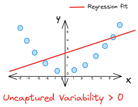
Imagine you have some dummy 2D data $(X, y)$. Now, in most cases, there will be some noise in the true outcome variable ($y$).
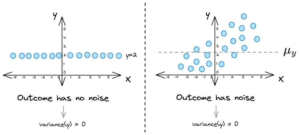
This means that the outcome has some variability, i.e., the variance of the outcome variable ($y$) is non-zero ($\sigma_{y} \ne 0$).
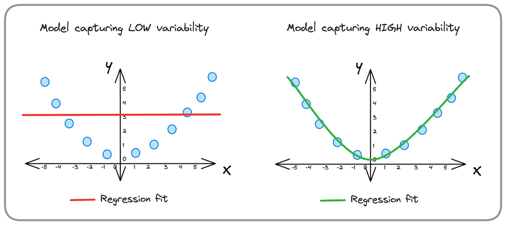
$R^{2}$ helps you precisely quantify the fraction of total variability in the outcome that the model is capturing.
Here lies an inherent assumption that a model capturing more variability is expected to be better than one capturing less variability.
Thus, we mathematically define $R^{2}$ as follows:
$$ R^{2} = \frac{\text{Variability captured by the model}}{\text{Total variability in the data}} $$
- $\text{Variability captured by the model}$ is always bounded between $[O, \text{Total variability in the data}]$.
- Thus, $R^{2}$ is always bounded between $[0,1]$.
A perfect $R^{2}$ of $1$ would mean that the model is capturing the entire variability.
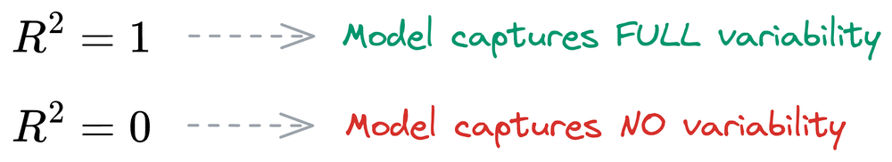
And an $R^{2}$ of $0$ would mean that the model is capturing NO variability. Such a model is obtained when you simply predict the mean value.
To recap, we define $R^{2}$ as follows:
$$ R^{2} = \frac{\text{Variability captured by the model}}{\text{Total variability in the data}} $$
Let’s consider the numerator and denominator separately now.
Total variability
As the name suggests, total variability indicates the variation that already exists in the data.
Thus, it can be precisely determined using the variance of the true outcome variable $(y)$, as shown below:
$$ \Large \text{Total variability} = \sum_{i=1}^{n} (y_{i} - \mu_{y})^2$$
This is commonly referred to as the Total Sum of Squares (TSS).
Variability captured by the model
Next, having trained a model, the goal is to determine how much variation is it precisely able to capture.
We can determine the variability captured by the model using the variability that is NOT captured by the model.
Essentially, variability captured and not captured should add to the total variability.
$$ {\text{Variability captured}} + {\text{Variability NOT captured}} = {\text{Total Variability}}$$
By rearranging, we get the following:
$$ {\text{Variability captured}} = {\text{Total Variability}} - {\text{Variability NOT captured}}$$
We have already determined the total variability above (also called TSS).
Next, we can define the variability not captured by the model as the squared distance between the prediction $(\hat y_{i})$ and the true label $(y_{i})$:
$$ {\text{Variability NOT captured by the model}} = \sum_{i=1}^{n} (\hat y_{i} - y_{i})^{2} $$
Why?
The term “Variability NOT captured by the model” represents the sum of squared differences between the predicted values $(\hat y_{i})$ and the actual values $(y_{i})$ of the dependent variable for all data points $(i=1, 2, ..., n)$.
It quantifies the amount of variation in the outcome variable that remains unexplained by the linear regression model.
For instance, in a perfect fit scenario, where the R-squared value is $1$, the predicted values $(\hat y_{i})$ must perfectly match the actual values $(y_{i})$ for all data points.

This results in a variability NOT captured by the model of $0$. In such a case, the model accounts for all the variation in the dependent variable, and there is no unexplained variability.
However, in cases where the R-squared value is less than $1$ (indicating a less-than-perfect fit), the predicted values $(\hat y_{i})$ might deviate from the actual values $(y_{i})$
Consequently, the variability NOT captured by the model increases, representing the amount of variance that remains unexplained by the model.
Thus, to recap, we can safely define the unexplained variance as follows:
$$ {\text{Variability NOT captured by the model}} = \sum_{i=1}^{n} (\hat y_{i} - y_{i})^{2} $$
The above is commonly referred to as the Residual Sum of Squares (RSS), which is also used in the Mean Squared Error (MSE) loss function in regression (considering the mean $\frac{1}{n}$ factor).