Why Do We Use Sigmoid in Logistic Regression?

👉

Introduction

Logistic regression is a regression model that returns the probability of a binary outcome ($0$ or $1$).

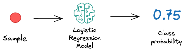
We all know logistic regression does this using the sigmoid function.

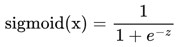
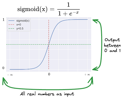
The sigmoid function maps any real-valued number $x \in \mathbb{R}$ to a value between $0$ and $1$. This ensures that output falls within a valid probability range.

While this may sound intuitive and clear, the notion of using Sigmoid raises a couple of critical questions.

Question #1: Of all possible choices, why Sigmoid?

An infinite number of functions can monotonically map a real input $(x)$ to the range $[0,1]$.

But what is so special about Sigmoid?

For instance, the figure below shows six possible alternative functions.

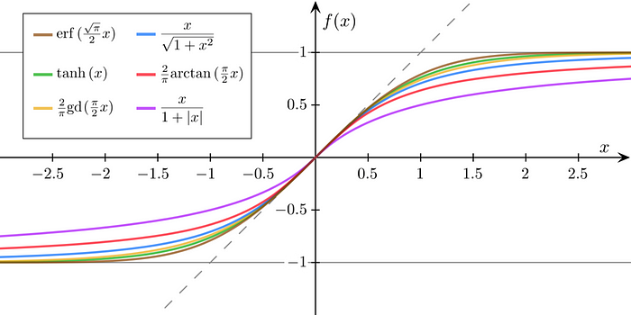
Alternatives to Sigmoid (Source: Activation function blog)

Note: While the output for the above functions is from $[-1, 1]$, we can squish it to [0,1] by scaling and shifting, as shown below:

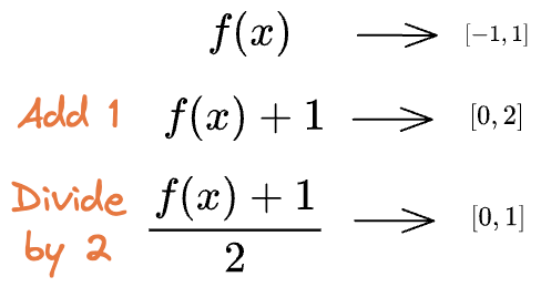
Yet, out of infinitely many choices, Why Sigmoid?

Question #2: How can we be sure that the output is indeed a probability?

The output of a logistic regression model is interpreted as a probability.

However, this seemingly straightforward notion raises an essential question: “Can we confidently treat the output of sigmoid as a genuine probability?”

See, it is important to consider that not every numerical value lying within the interval of $[0, 1]$ guarantees that it represents a legitimate probability.

In other words, just outputting a number between $[0, 1]$ isn't sufficient for us to start interpreting it as a probability.

Instead, the interpretation must stem from the formulation of logistic regression and its assumptions.

Thus, in this article, we'll answer the above two questions and understand the origin of Sigmoid in logistic regression.

Going ahead, we'll also understand the common categorization of classification approaches and takeaways.

Let's begin!

Why Sigmoid? – Answers from the web

Before understanding the origin of the sigmoid function in logistic regression, let's explore some of the common explanations found on the web.

Incorrect Explanation #1

The most profound explanation is providing no explanation at all. In other words, most online resources don't care to discuss it.

In fact, while drafting this article, I did a quick Google search, and disappointingly, NONE of the top-ranked results discussed this.

*Results for “Logistic Regression Guide”*

The sigmoid function is thrown out of thin air along with its plot.

And its usage is justified by elaborating that Sigmoid squishes the output of linear regression between $[0,1]$, which depicts a probability.

A couple of things are wrong here:

It conveys a misleading idea that logistic regression is just linear regression with a sigmoid. Although the definition does fit in pretty well mathematically, this is not true.
They didn't elaborate on “why sigmoid function?” Even if we consider the flawed reasoning of squishing the output of linear regression to be correct for a second, why not squish it with any other function instead?

Incorrect Explanation #2

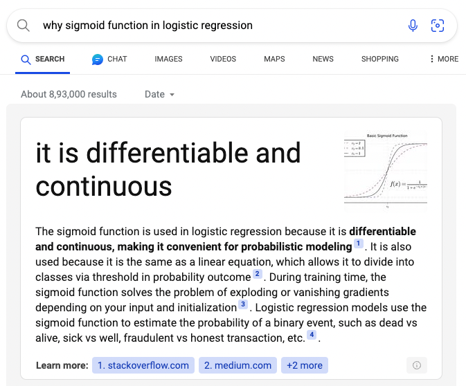
Another inaccurate answer was generated from the search query above.

Let's look at what's wrong with this explanation.

The answer says, "It is differentiable and continuous."
- Counterpoint: There are infinitely many functions that can be differentiable and continuous. Why Sigmoid?
The answer says, "During training time, the sigmoid function solves the problem of exploding or vanishing gradients depending on your input and initialization."
- Counterpoint: The rationale of vanishing and exploding gradient only makes sense in neural networks. This has nothing to do with logistic regression.
The answer says: "Logistic regression models use the sigmoid function to estimate the probability of a binary event, such as dead vs.. alive, sick vs well, fraudulent vs. honest transaction, etc."
- Our counterpoint: How do we prove that it models a probability? There are infinitely many functions that map can potentially map the output to $[0,1]$, which can be possibly interpreted as a probability. What makes Sigmoid special?

Incorrect Explanation #3

Some answers derive the sigmoid equation from the fact that logistic regression is used to model “log odds.”

Let's understand “log odds” first.

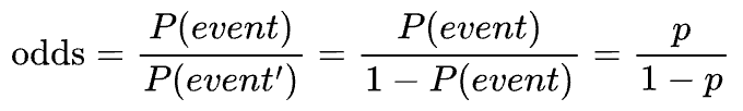
In probability, “odds” is defined as the ratio of the probability of the occurrence of an event $(P(event))$ and the probability of non-occurrence $(1-P(event))$.

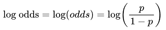
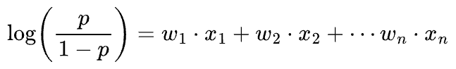
“Log odds,” as the name suggests, is the logarithm of odds, as shown below:

These answers convey that logistic regression is used to model log odds as a linear combination of the features.

Assuming $X = (x_{1}, x_{2}, \cdots, x_{n})$ as the features and $W = (w_{1}, w_{2}, \cdots, w_{n})$ as weights of the model, we get:

log odds as a linear combination of features

Exponentiating both sides and solving for $p$, we get:

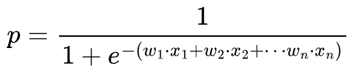
This is precisely the sigmoid function.

While this may sound convincing, there are some major flaws here.

How do we know that logistic regression models log odds?
In reality, it is only when we derive the sigmoid function that we get to know about log odds. Thus, the “log odds” formulation is mathematically derived from the sigmoid representation of logistic regression, not the other way around. But this answer took the opposite approach and assumed that logistic regression is used to model log odds.

By now, you must be convinced that there are some fundamental misalignments in proving the utility and origin of the sigmoid function in the above explanations.

There are some more incorrect explanations here:

Most individuals are introduced to the Sigmoid function using one of the above explanations.

But as discussed, none of them are correct.

In my opinion, an ideal answer should derive logistic regression in terms of Sigmoid from scratch and with valid reasoning.

Thus, one should not know anything about it beforehand.

It is like replicating the exact thought process when a statistician first formulated the algorithm by approaching the problem logically, with only probability and statistics knowledge.

Ready?

Let's dive in!

Why Sigmoid?

Sigmoid Notebook

The code accompanying the experiments conducted in this article.

Why sigmoid.ipynb

388 KB

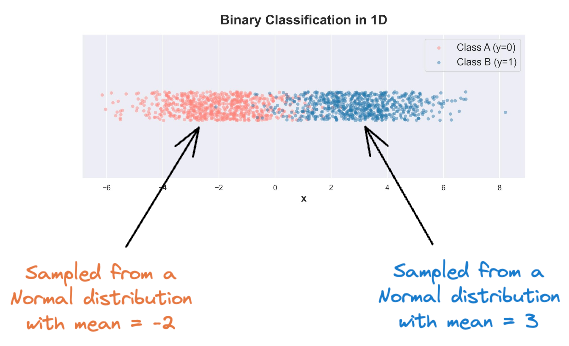
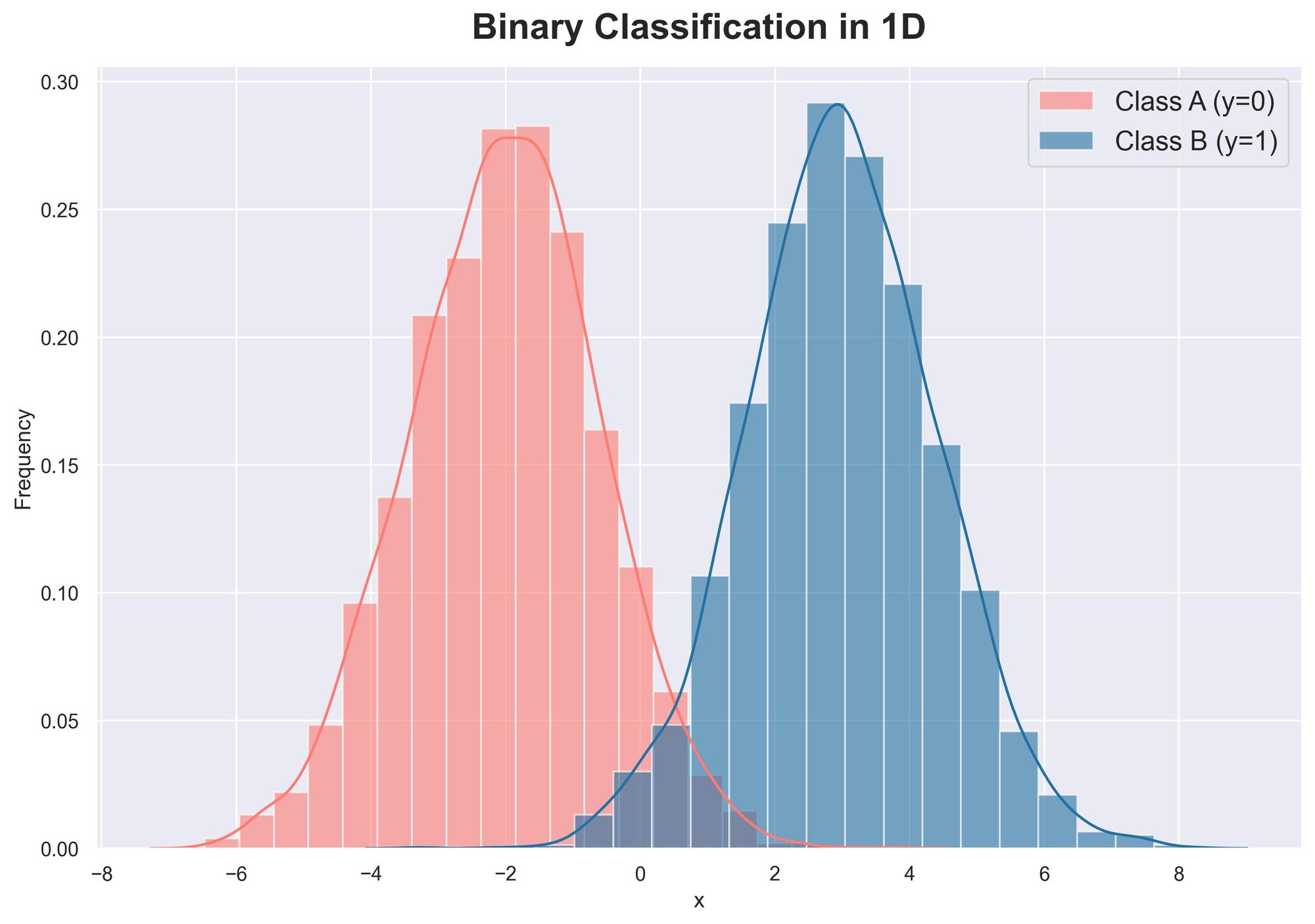
For simplicity, consider the following binary classification data in one dimension:

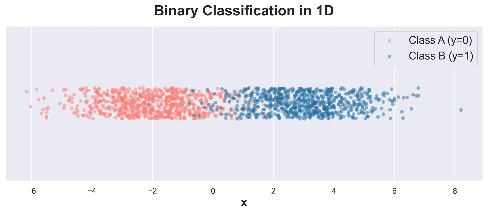
Both classes have an equal number of data points ($n$). Also, let's assume that they were sampled from two different normal distributions with the same variance $\sigma=1$ and different mean ($-2$ and $3$).

Binary classification dummy data sampled from two different normal distributions

Plotting the class-wise distribution (also called the class-conditional distribution), we get:

Class-conditional distribution (KDE + Histogram) of the dummy data

Being 1-dimensional data, it is easy to visually fit a vertical decision boundary that separates the two classes as much as possible.

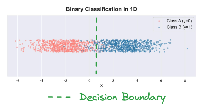
Let's see if we can represent this classification decision mathematically.

Essentially, the objective is to predict the probability of each class given an input.

Probability of a specific class given an input

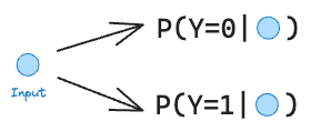
Once we do that, we can classify a point to either of two classes based on whichever one is higher.

Now, what information do we have so far:

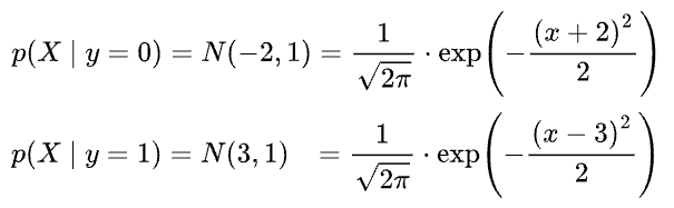
We know the class conditionals $p(X|y=1)$ and $p(X|y=0)$, which are Gaussians. These are the individual distributions of each class.
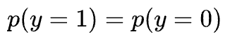
We know the priors $p(y=1)$ and $p(y=0)$. We assumed that both classes have equal data points ($n$). Thus, prior is $\frac{1}{2}$ for both classes.

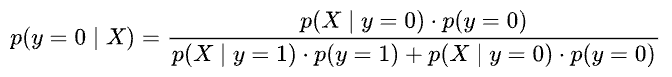
With this info, we can leverage a generative approach for classification.

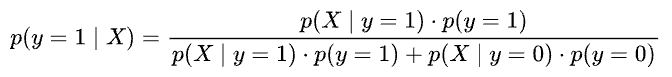
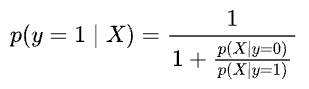
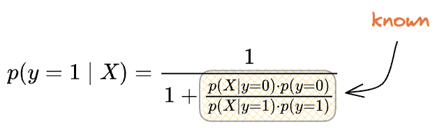
As a result, we can use the Bayes rule to model the posterior $p(y=0|X)$ as follows.

💡

$p(y=0|X)$ is read as follows: The probability that the output label is 0, given an input X. This is also called posterior probability.

And $p(y=1|X)$ as follows:

Plotting both posteriors over a continuous range of $X$, we get:

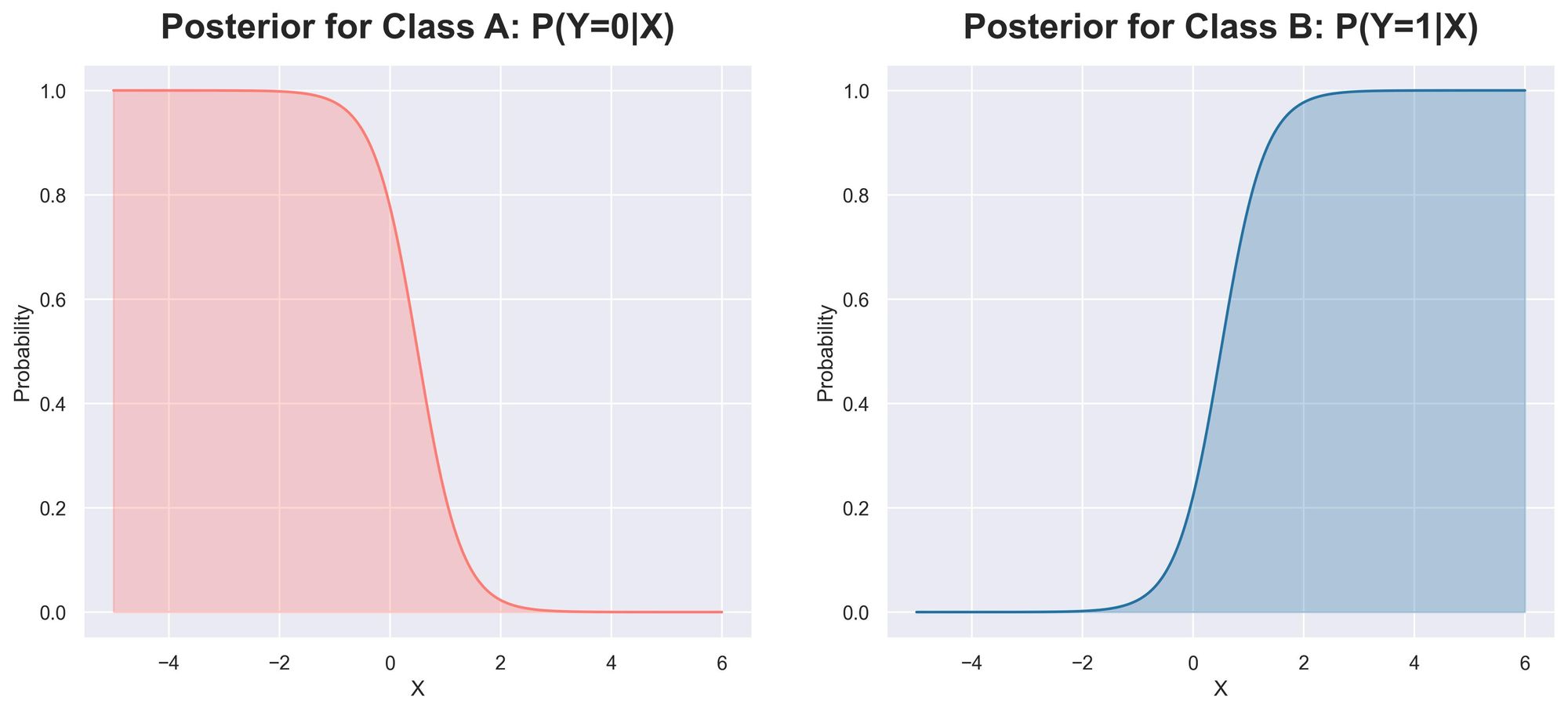
Posterior probabilities for Class A and Class B

Alternatively, we can merge them into a single plot.

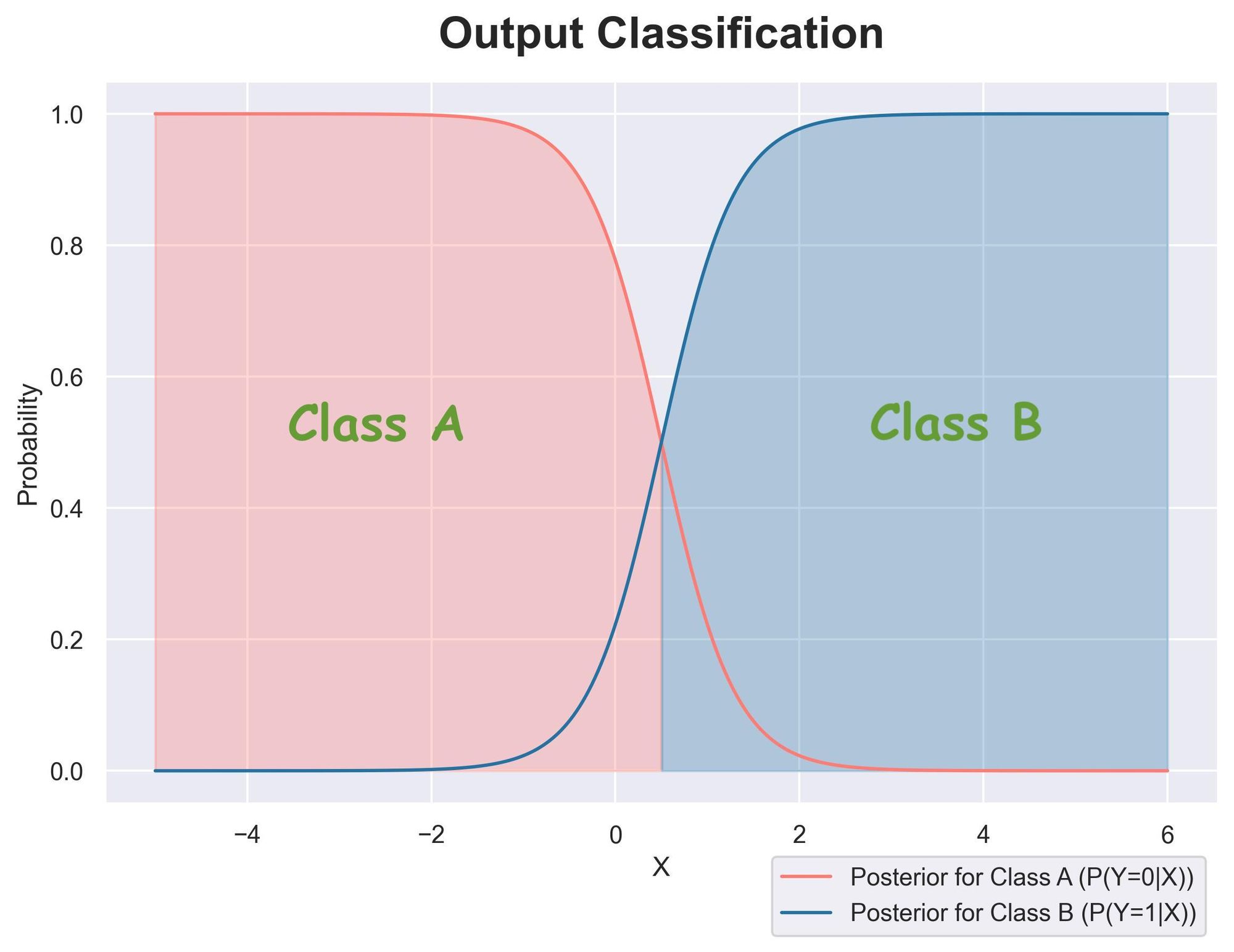
Posterior probabilities for Class A and Class B in a single plot

In the above plot:

There's a clear decision boundary.
The light pink region indicates that the posterior for "Class A" is higher. This means that $p(y=0|X) > p(y=1|X)$. Thus, the sample is classified as "Class A."
The blue region indicates that the posterior for "Class B" is higher. This means that $p(y=1|X) > p(y=0|X)$. Thus, the sample is classified as "Class B."
Both posteriors always add to $1$. This is because the Bayes theorem normalizes them.

💡

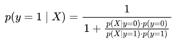
On a side note, if we consider the posterior probability curve of the Blue class ("Class B") which is represented by the S shape, it does look like the sigmoid shape we are looking for. Yet, let's not assume it is a Sigmoid and instead, derive it.

Let’s derive the posterior for “Class B” by substituting the relevant values:

We distribute the numerator to the denominator:

Now, we assumed the priors to be equal:

Equal priors

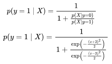
Thus, we get:

Also, we assumed the class conditionals to be Gaussians with the same variance ($\sigma=1$) and different mean ($-2$ and $3$):

Substituting back in the posterior for “Class B,” we get:

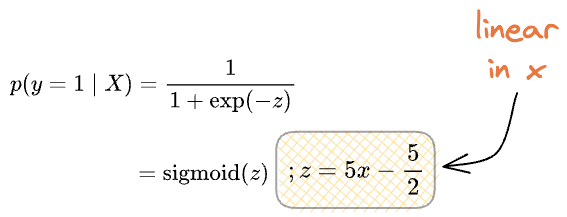
Simplifying further, we get the following:

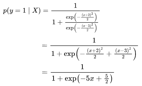
Assuming $z = 5x-\frac{5}{2}$, we get:

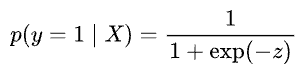
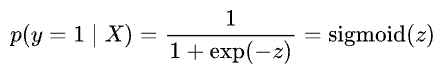
And if you notice closely, this is precisely the sigmoid function!

Once we have Sigmoid, we can obtain its inverse by solving for $z$:

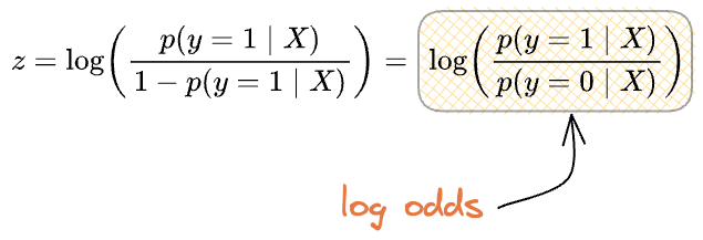
And that’s how we get to know that logistic regression models log odds.

Now recall all the incorrect reasonings we discussed above and how misleading they were.

This derivation also answers the two questions we intended to answer:

"Of all possible choices, why sigmoid”: Because it comes naturally from the Bayes rule for two classes, where the target variable has a Bernoulli distribution.
"How can we be sure that the output is a probability?”: Because we used the bayes rules to model the posterior, which is precisely used to determine the probability of an event.

The above formulation of Sigmoid also lets us translate a generative model to a discriminative model, both of which are widely used in classification problems.

If you don’t know what they are, here’s a quick refresher.

Discriminative and Generative models

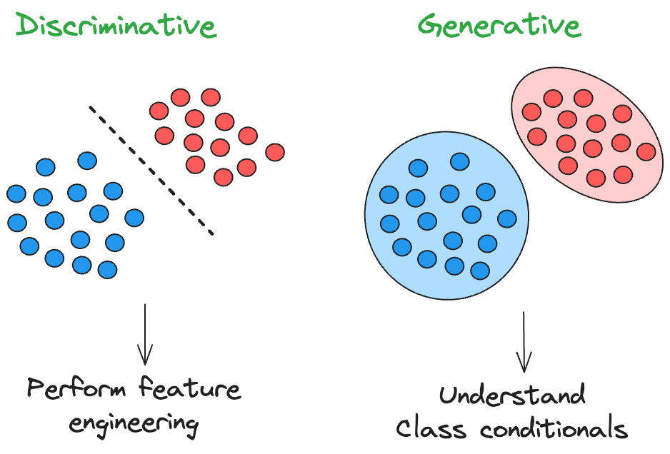
In general, classification models can be grouped into two categories: discriminative models and generative models.

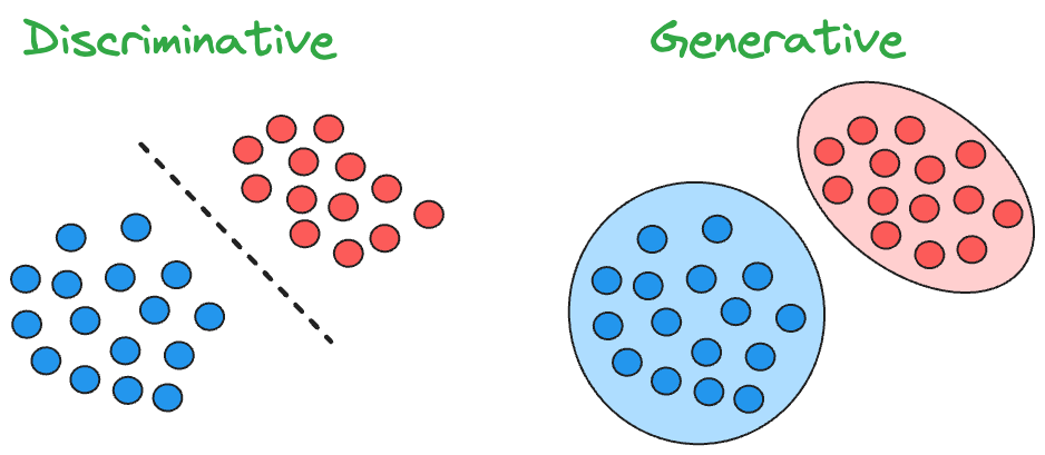
Discriminative models learn the decision boundaries between the classes, while generative models learn the input distributions for each class.

In other words, discriminative models directly learn the function $f(x)$ that maps an input vector ($x$) to a label ($y$).

This may happen in two ways:

They may try to determine $f(x)$ without using any probability distribution. They assign a label for each sample directly, without providing any probability estimates, such as decision trees and SVM.
They may learn the posterior class probabilities $P(y = k|x)$ first from the training data. Based on the probabilities, they assign a new sample $x$ to the class with the highest posterior probability, such as logistic regression and neural networks.

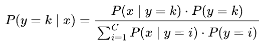
Whereas, generative models first estimate the class-conditional densities $P(x|y = k)$ and the prior class probabilities $P(y = k)$ from the training data.

Then, they estimate the posterior class probabilities using Bayes’ theorem:

Examples of generative models are:

Naive Bayes
Gaussian mixture models (GMMs)
Hidden Markov models (HMMs)
Linear discriminant analysis (LDA), etc.

If that is clear, let's dive back into the Sigmoid derivation.

Breaking the assumptions

The derivation of the posterior estimation above gave us an expression in the linear form of $x$ before applying Sigmoid.

The posterior probability is the Sigmoid of a linear term of x

This happened because we assumed two Gaussians with:

Same priors ($p(y=1)$ and $p(y=0)$)
Same variance $(\sigma)$

...and this allowed us to cancel the quadratic term of x that would have appeared otherwise, as shown below.

What would happen if the distributions had:

Different priors
Different variance

For instance, consider two dummy 2D classification datasets.

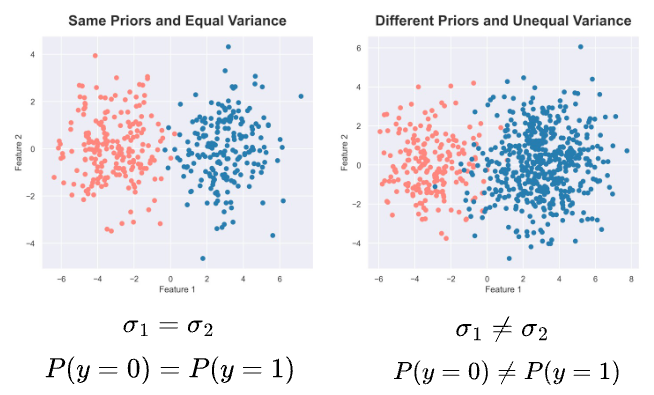
Left: 2D dummy data with equal variance and priors. Right: 2D dummy data with unequal variance and priors.

On the left, each class has the same number of samples (i.e., same priors) and is generated using a normal distribution of equal variance.

On the right, each class has a different number of samples (i.e., different priors) and is generated using a normal distribution of unequal variance.

What information do we have:

We know the class conditionals $p(X|y=1)$ and $p(X|y=0)$, which are Gaussians.
Although unequal, we know the priors $p(y=1)$ and $p(y=0)$.

As a result, we can still leverage a generative approach for classification and use Bayes’ rule to model the posterior $p(y=1|X)$ as follows.

Plotting the decision boundary obtained using Bayes’ rule, we get:

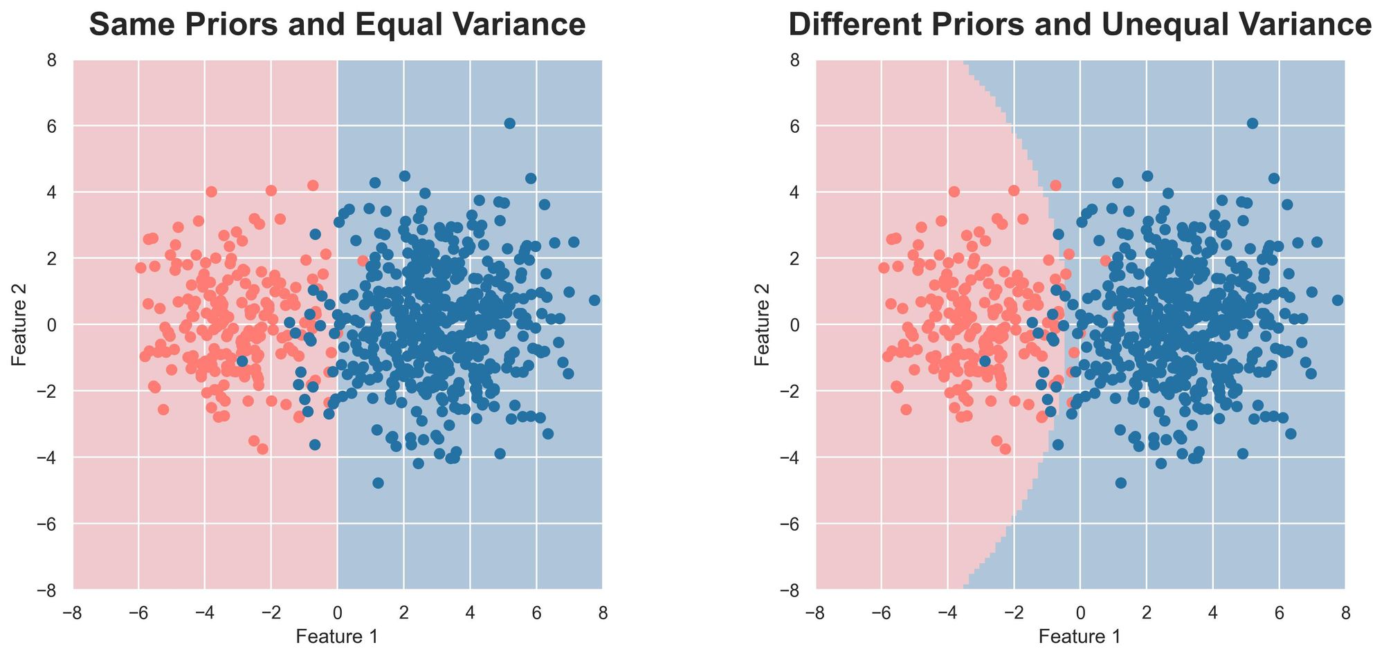
Decision regions obtained using Bayes' rule

The decision boundary is linear if the two Gaussians have the same variance (this is called covariance matrix for non-1D dataset) and equal priors.

However, if they have different covariance matrices, the decision boundary is non-linear (or parabolic), which also makes sense.

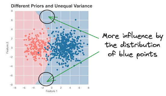
It is expected because the normal distribution that generated the blue data points has a higher variance.

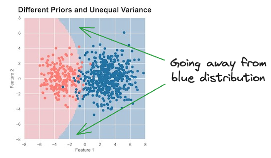
This means that its data points are more spread out, and thus, it has a large area of influence than the left one.

The distribution of blue data points has more variance. Thus, they have more influence.

The essence is that with unequal variance and different priors, the squared term will not cancel out. The priors won't cancel out either.

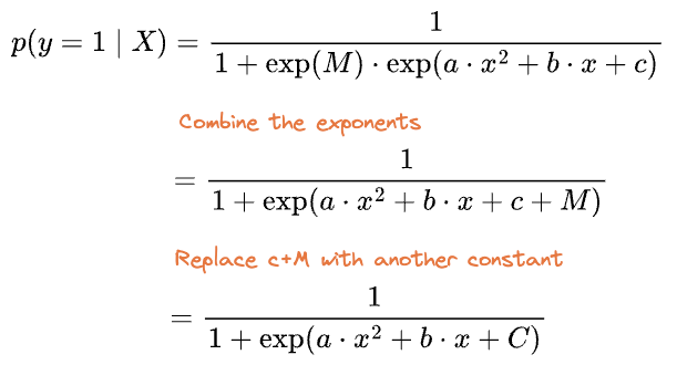
Thus, the final posterior probability estimation must look like this:

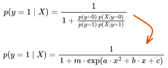
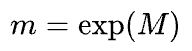
Here, $m$ is the ratio of the priors, which is always positive. Thus, it can be represented as the exponent of some other constant $M$.

Simplifying, we get:

Now, let’s try to model these two dummy classification datasets with logistic regression using its 2D features (i.e., a discriminative approach).

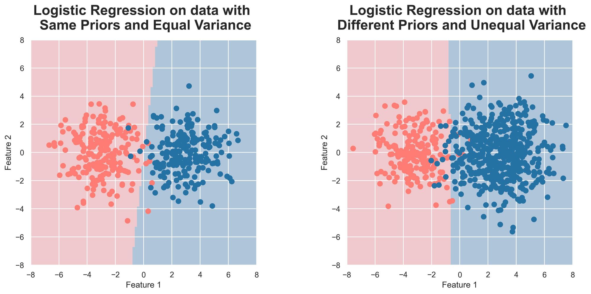
Decision regions obtained using Logistic Regression

Did you notice something?

In contrast to the generative approach, both decision regions are linearly separated, which is not entirely correct.

This was expected because we modeled the data without any polynomial features.

In other words, while modeling the data with logistic regression, we did this:

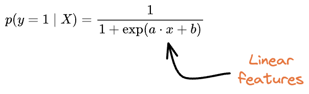
But due to unequal variance and different priors in this 2D dataset, we saw from the generative approach that polynomial features were expected:

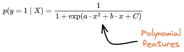
Had we engineered the features precisely, it would have resulted in a similar decision boundary as obtained with the generative approach.

Nonetheless, we also had an advantage when using logistic regression.

In this case, we modeled the data without prior information about the data generation process, which was necessary for the generative approach.

This indicates that if we model the posterior directly with a discriminative approach or understand the class conditionals first to use a generative approach, both have some pros and cons.

Let’s understand!

Generative vs. Discriminative

In classification tasks, the choice between generative and discriminative models involves trade-offs.

In the generative framework, one crucial prerequisite is the prior knowledge of the class conditionals and priors.

For instance, when we used the generative approach above, we had prior info about them.

Here, while priors are directly evident from the data – just count the occurrence of each label, class conditionals, at times, may demand effort and understanding of the data.

But once the generative process is perfectly understood, accurate modeling automatically follows.

In contrast, discriminative approaches focus on modeling the posterior probabilities $(p(y=1|X)$) directly.

But the effort of estimating the class conditionals in a generative approach translates to feature engineering in the discriminative framework.

Thus, understanding the trade-offs between these approaches is essential in choosing an appropriate model for a given classification problem.

Takeaways

Discriminative models learn the decision boundary between classes. Generative models understand the underlying data distribution.
Discriminative models are often faster to train. Yet, they may not perform as well on tasks where the underlying data distribution is complex or uncertain. This requires extensive feature engineering.

In general:

Generative models impose a much stronger assumption on the class conditionals (or require prior info about the distribution). But when we know the distribution, it requires less training data than discriminative models.
When the assumption of class conditionals is not certain, discriminative models do better. This is because they don’t need to model the distribution of the features. However, this does require extensive feature engineering.

Conclusion

In my experience, in most courses/books/tutorials, solutions are always introduced cleverly without giving proper reasoning and justification.

The same is the case with introducing the Sigmoid function in logistic regression.

While these resources teach the “how” stuff, it is only when we get to know the “why” stuff that we can confidently apply those learnings to real-life applications.

Thus, a solid understanding of the underlying concepts is foundational to validate their practical applicability.

It also benefits us in developing new approaches by addressing the limitations of existing ones.

But that is only possible when the foundational knowledge is learned perfectly.

This is precisely what we intend to distill in these weekly deep dives, which you mind interesting to read next: