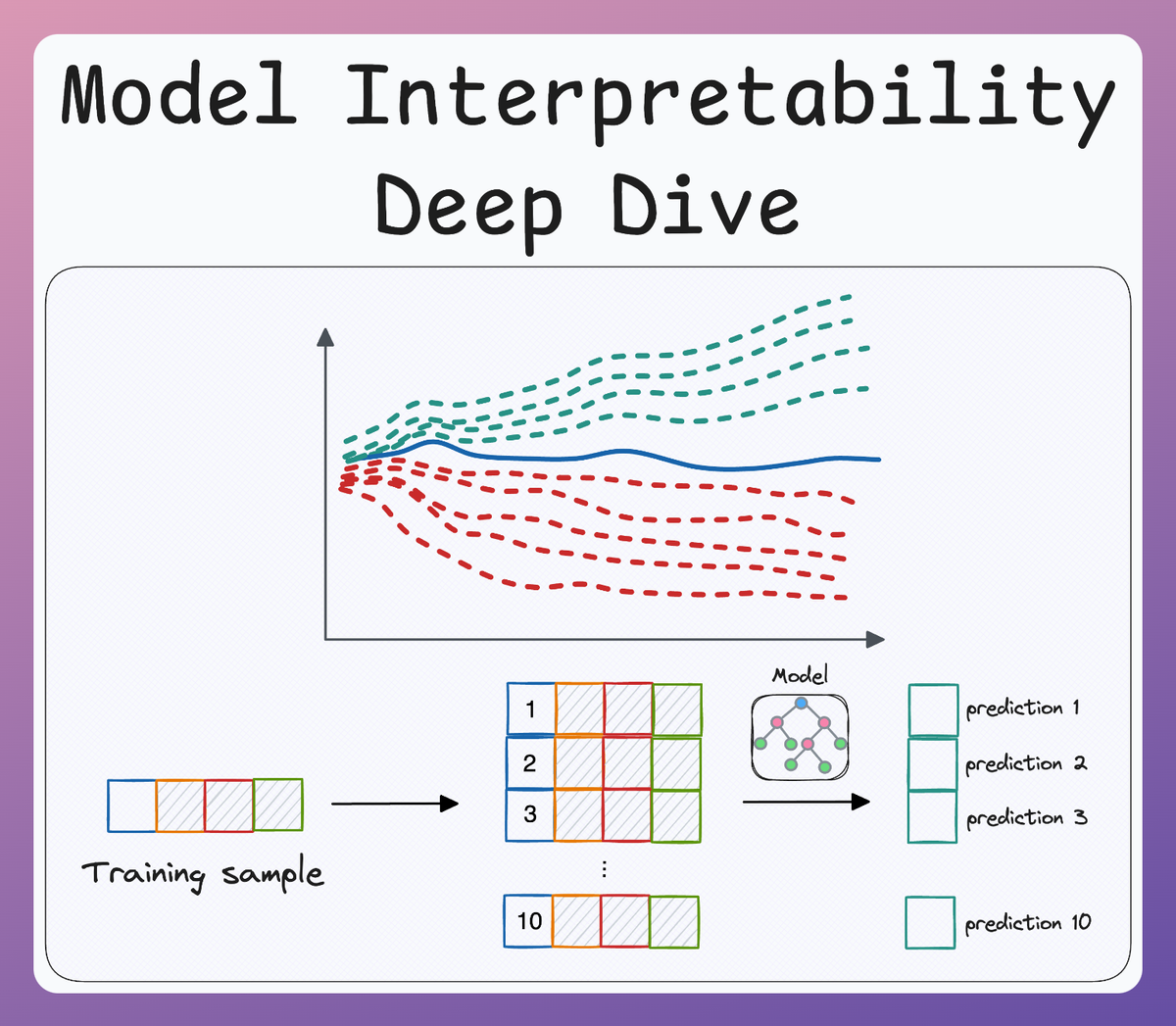
Model Interpretability (Part 3)
A deep dive into interpretability methods, why they matter, along with their intuition, considerations, how to avoid being misled, and code.
Introduction
Over the last couple of weeks, we have been extensively covering topics around building interpretable machine learning (ML) models.
- In the first part of this crash course, we went into quite a lot of detail about some model interpretability methods and how Partial Dependence Plots (PDPs) and Individual Conditional Expectation (ICE) help us investigate the predictions of a machine learning model:
- In Part 2, we covered some of the limitations of the methods discussed in Part 1 and how LIME addresses those. More specifically, unlike traditional methods that produce insights into the overall trend of the model, LIME takes a local approach, so we get to have interpretable explanations for individual predictions.

Towards the end of Part 2, one thing we noticed was that the LIME weights for each feature DO NOT belong to the complex model but rather the coefficients of the surrogate model.
As a result, the sum of the weights of the surrogate model at the current instance will likely not be equal to the actual prediction for the given instance.
We also verified this using the code below.
First, we selected a random instance and generated a prediction from the complex random forest model:
Next, we summed the LIME feature contributions (coefficients of the surrogate model) and the intercept term to get the prediction from the surrogate model:
It is clear that actual prediction (3.94) and the one from the surrogate model (4.7) differ.
I would recommend reading Part 1 and Part 2 if you haven't already before reading this deep dive:
Since the two predictions did not match, this may not be a desirable property and we may want our explainer to be as close to the true prediction as well.
This is a property that SHAP satisfies, which makes SHAP values much more dependable in that respect.
Like in Part 2, let's dive into the technical details of how SHAP works internally and how to interpret it (while ensuring that they don't mislead you).
Let's begin!
Real-life analogy of Shapley values
If you have ever heard about SHAP before, one thing that you would typically find people associating it with is "Shapley." First, let's understand what it is and why they are so foundational to SHAP.
Scenario: 2-person business
Let’s say you and your friend start a business together.

At the end of the year, the business makes \$100,000 in profits, and now you need to figure out how to split this money fairly.

However, while you both contributed to the success of the business, your friend suggests splitting the money equally, but you feel that your contribution was higher, and you should receive a larger share.
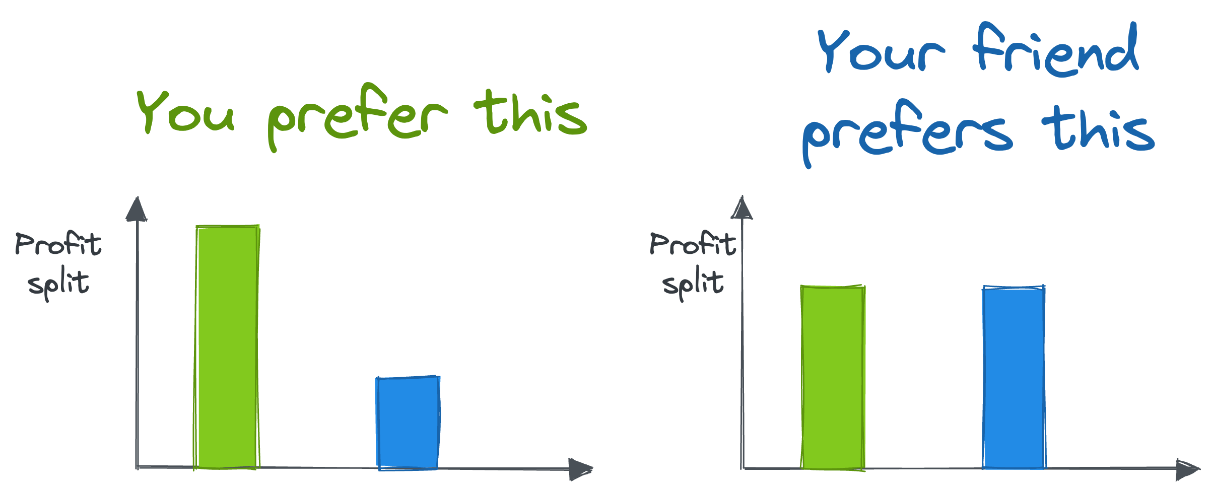
Don't you think an intuitive way to divide the profits fairly is by considering how much each of you contributed to the success of the business?
So here’s how the Shapley value can help you fairly divide the profits based on each person’s marginal contribution to the business.
Step 1: Evaluate profits from different coalitions
Imagine we have a way to determine how much money the business would have made if each person had worked alone, and how much the business makes when you both work together.
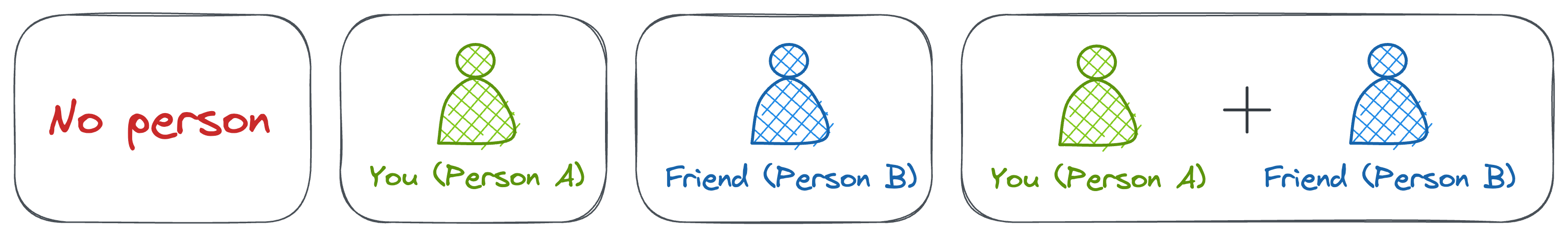
Here's what it looks like:
- Both you and your friend work together, and the business makes \$100,000.
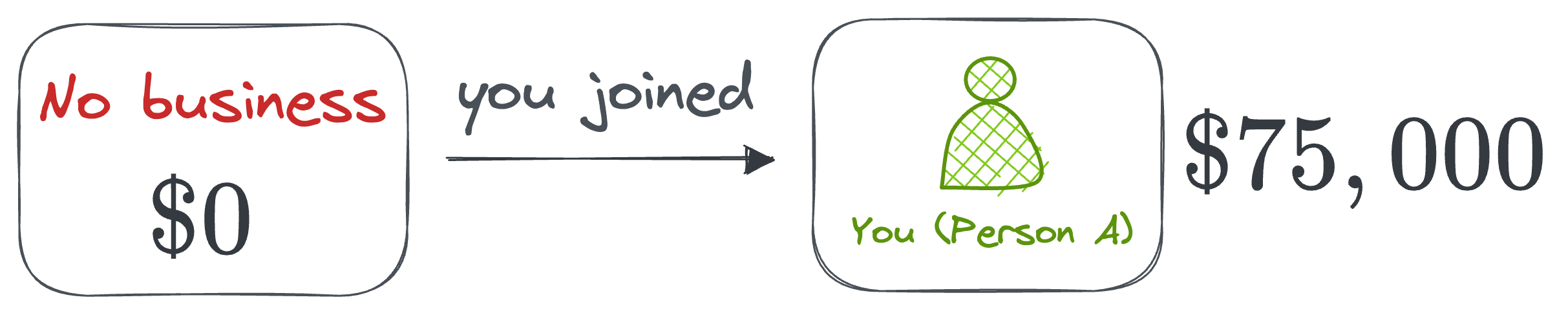
- You alone (without your friend) would have made \$75,000 in profit.
- Your friend alone (without you) would have made \$50,000.
- If neither of you were involved, the business would make \$0 (no business, no profit).
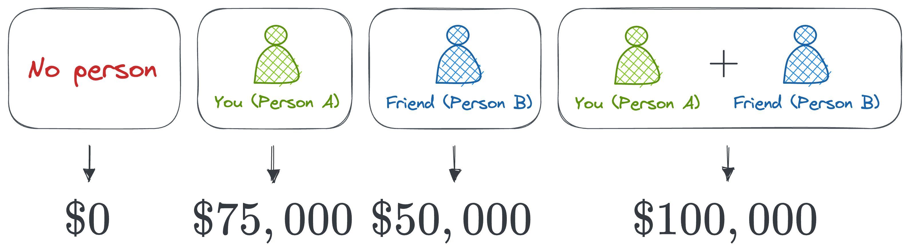
This gives us four possible coalitions and the respective profits generated.
Step 2: Calculate the Marginal Contributions
To calculate the Shapley value, we need to determine each person’s marginal contribution to the profit.
This is the additional profit that each person brings to the business when they join a coalition.
Your marginal contribution (Person A)
- When you join the business alone (no friend involved), you make \$75,000. Since the coalition without you made \$0, your marginal contribution is \$75,000.
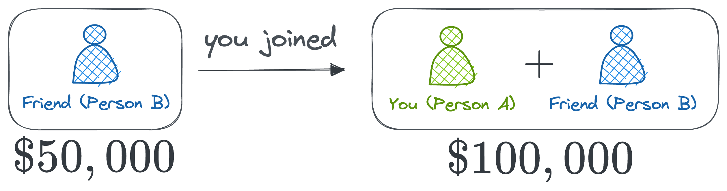
- When you join the business when your friend is already in the coalition (your friend would have made \$50,000 alone), the profit increases from \$50,000 to \$100,000. So, your marginal contribution in this scenario is \$50,000.
Your friend's marginal contribution (Person B)
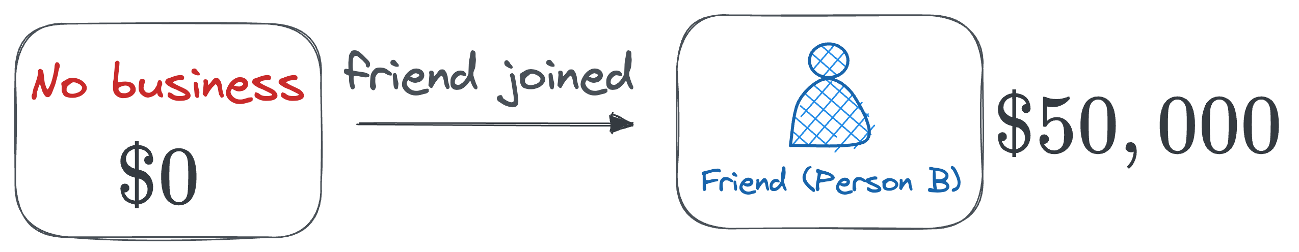
- When your friend works alone, they make \$50,000. Since the coalition without them made \$0, their marginal contribution is \$50,000.
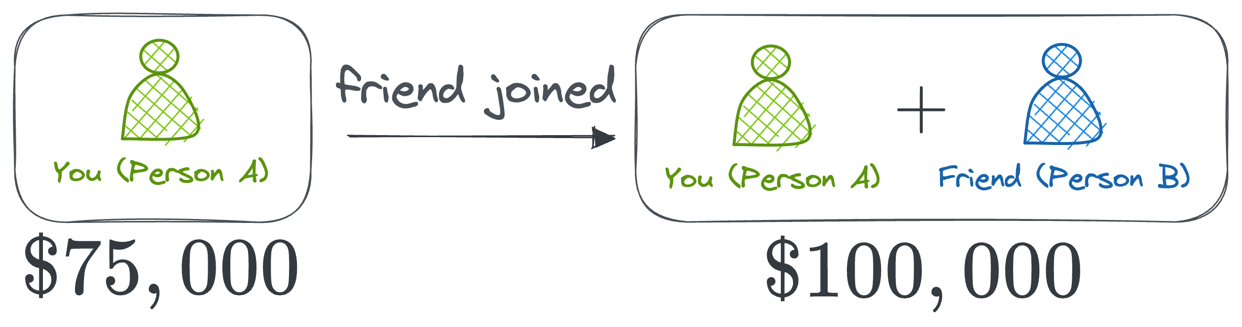
- When your friend joins the business while you’re already part of it (you would make \$75,000 alone), the profit increases from \$75,000 to \$100,000. So, their marginal contribution in this scenario is \$25,000.
Step 3: Calculate the Shapley values
To fairly split the profits, we take the average of the marginal contributions across all possible coalitions. This gives us the Shapley value for each person.
Your Shapley value (Person A)
- Your marginal contribution when working alone: \$75,000.
- Your marginal contribution when joining your friend: \$50,000.
- We average your marginal contributions to get your Shapley value: