15 Ways to Optimize Neural Network Training (With Implementation)

Introduction

I don’t think I have ever been excited about implementing (writing code) a neural network — defining its layers, writing the forward pass, etc.

In fact, this is quite a monotonous task for most machine learning engineers.

For me, the real challenge and fun lie in optimizing the network.

It’s where you take a decent model and turn it into a highly efficient, fine-tuned system capable of handling large datasets, training faster, and yielding better results.

It’s a craft that requires precision, optimization, and a deep understanding of the hardware and software involved.

That is why I never considered being able to train ML models to be a core skill.

Instead, it was always about understanding the science behind the model and applying the right techniques to get the most efficient results.

In this article, let me walk you through 15 different ways you can optimize neural network training, from choosing the right optimizers to managing memory and hardware resources effectively.

Each technique is backed by code examples to help you implement these optimizations in your own projects.

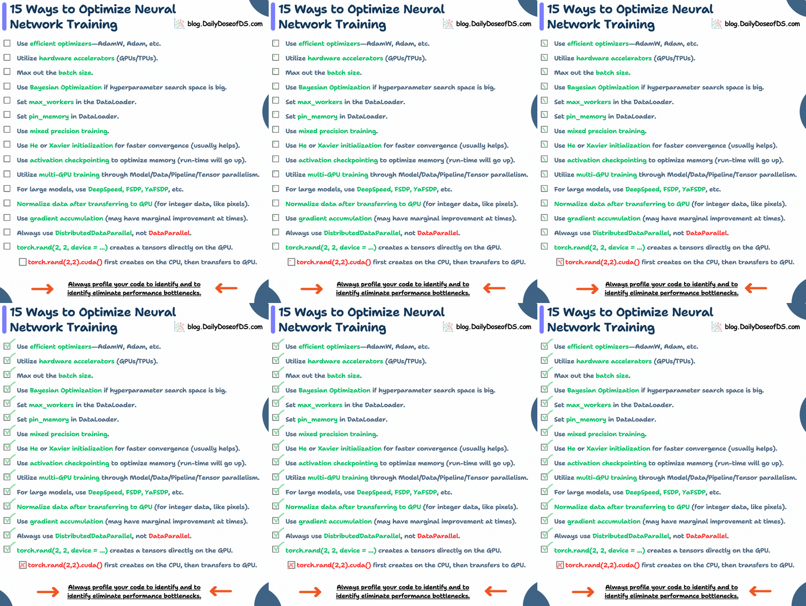
As you can tell from the animation above, some of these techniques are pretty basic and obvious, like:

• Use efficient optimizers—AdamW, Adam, etc.
• Utilize hardware accelerators (GPUs/TPUs).
• Max out the batch size.

So we won't discuss them here.

Let's begin!

#4-5) Max workers and pin memory

Max workers

Setting num_workers in the PyTorch DataLoader is an easy way to increase the speed of loading data during training.

The num_workers parameter determines how many subprocesses are used to load the data in parallel.

By increasing the number of workers, you can often significantly reduce data loading time, especially when dealing with large datasets.

In practice, this helps prevent the GPU from waiting for the data to be fed to it, thus ensuring that your model trains faster.

However, the optimal value for num_workers can depend on the specific machine you're using (CPU cores, RAM, etc.), so it’s recommended to experiment with different values.

Max workers implementation

To demonstrate effectiveness, let's consider a simple implementation involving a feedforward neural network on the MNIST dataset.

We begin with some standard imports and declare the device as follows:

Next, we define our feedforward neural network architecture:

Moving on, we define the MNIST dataset object:

Since we would be testing the performance of a standard dataloader against the one with multiple workers, let's define a method to do that:

This train function is a typical PyTorch training loop used for a neural network model. Here's a breakdown

• Parameters:
  • model: The neural network model to be trained.
  • device: The device (CPU or GPU) to which the tensors (data) should be moved for computation.
  • train_loader: The DataLoader that provides batches of training data.
  • optimizer: The optimization algorithm (e.g., Adam, SGD) used to update the model parameters.
  • criterion: The loss function (e.g., CrossEntropyLoss) is used to calculate the error between the predicted output and the target.
  • epoch: The current training epoch (iteration over the entire dataset).
• Next, we have the standard training procedure where it trains the model for one epoch, processing data in batches. It performs forward propagation to generate predictions, calculates the loss, performs backpropagation to compute gradients, and updates the model's parameters using the optimizer. The total loss for the epoch is printed at the end.

Standard data loader

First, let's experiment with a standard dataloader object first.

To do that, we first define the model, the loss function, and the optimizer:

Next, we create our standard data loader object and invoke the train method defined earlier:

As depicted above, the model takes about 43 seconds to train for five epochs.

Data loader with max workers

Next, let's experiment with another dataloader by specifying the max_workers parameter.

To do that, we again define the model, the loss function, and the optimizer:

Next, we create the data loader object and invoke the train method defined earlier:

As depicted above, the model follows almost the same loss trajectory but now takes
~10 seconds to train for five epochs, which is a massive reduction in training time.

By using multiple workers, the DataLoader can fetch data batches asynchronously, significantly improving training speed, especially for large datasets or when data preprocessing is required.

Pin memory

To understand this, consider the standard model training loop in PyTorch, as shown below:

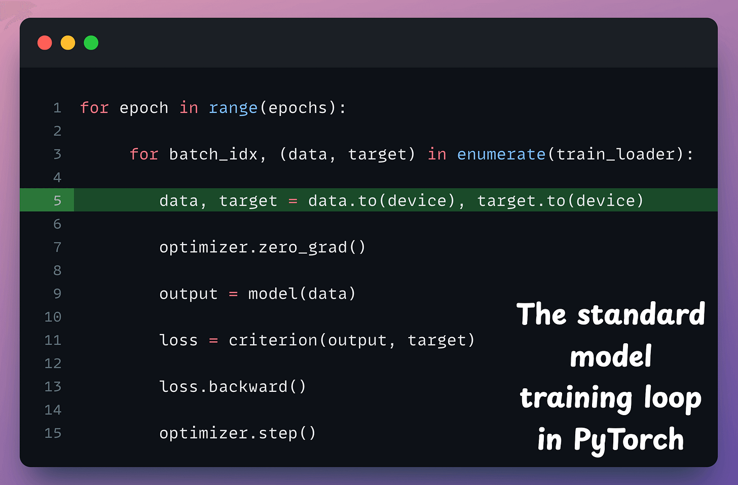
In the above code:

• Line 5 transfers the data to the GPU from the CPU.
• Everything executes on the GPU after the data transfer, i.e., lines 7-15.

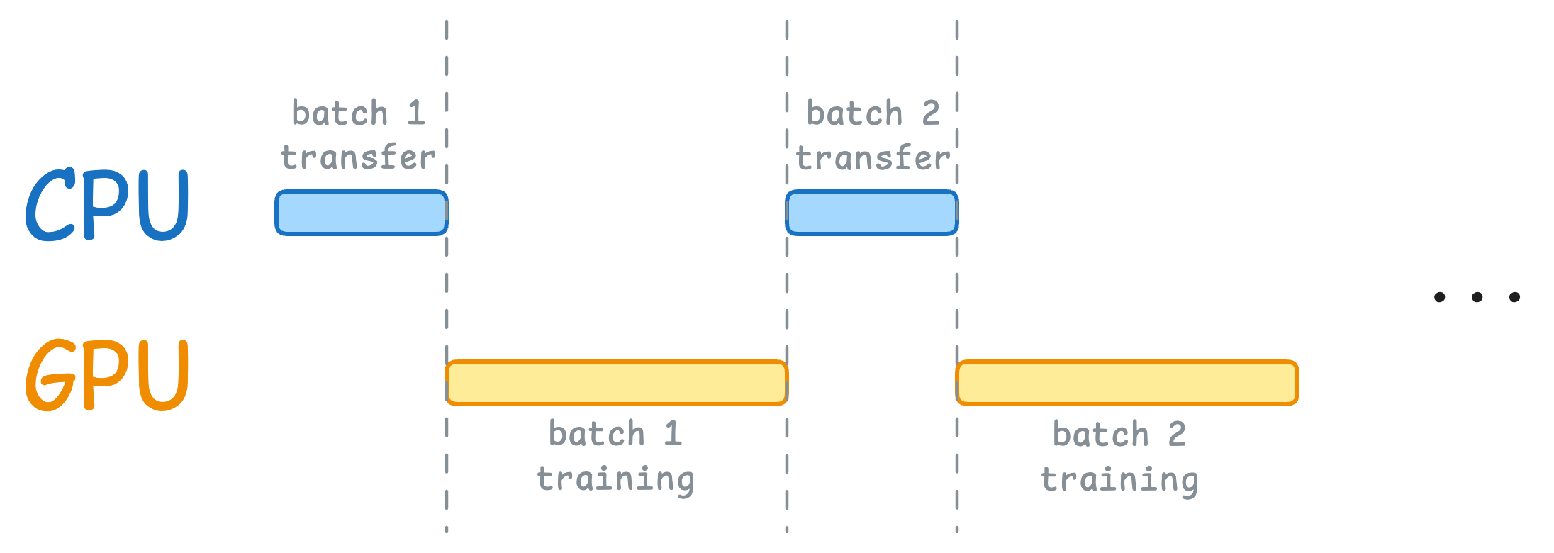
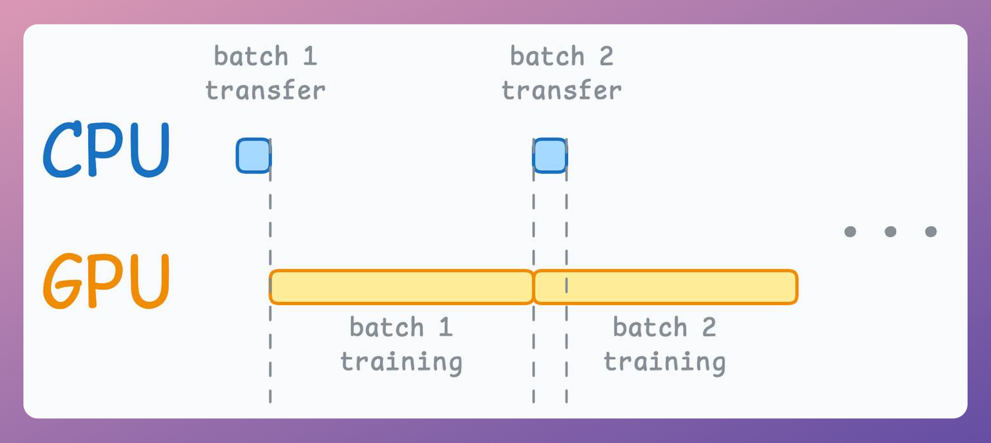
This means when the GPU is working, the CPU is idle, and when the CPU is working, the GPU is idle, as depicted below:

But here’s what we can do to optimize this:

• When the model is being trained on the 1st mini-batch, the CPU can transfer the 2nd mini-batch to the GPU.
• This ensures that the GPU does not have to wait for the next mini-batch of data as soon as it completes processing an existing mini-batch.

Thus, the resource utilization chart will look something like this:

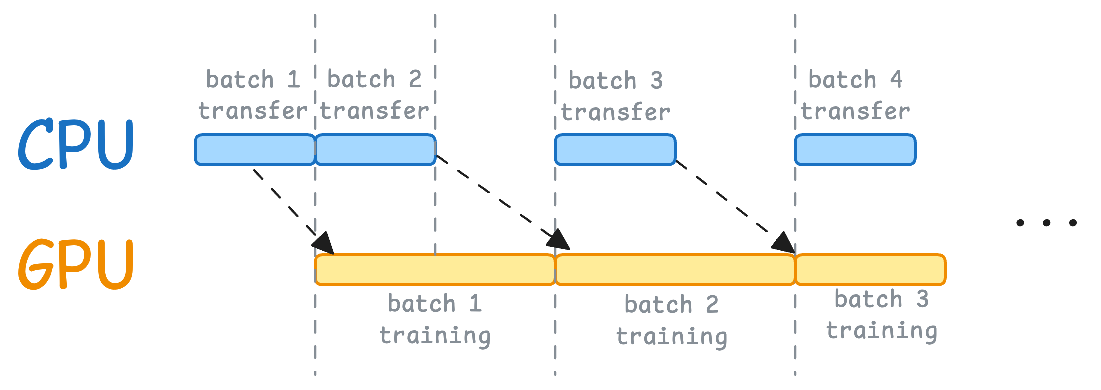
While the CPU may remain idle, this process ensures that the GPU (which is the actual accelerator for our model training) always has data to work with.

Formally, this process is known as memory pinning, and it is used to speed up the data transfer from the CPU to the GPU by making the training workflow asynchronous.

This allows us to prepare the next training mini-batch in parallel to training the model on the current mini-batch.

Enabling this is quite simple in PyTorch.

Essentially, setting pin_memory=True in the DataLoader ensures that the data is transferred directly to the GPU from pinned memory (memory that is page-locked), which is faster than transferring data from regular CPU memory.

Pin memory implementation

Firstly, when defining the DataLoader object, set pin_memory=True as depicted below:

Next, go back to the train() method we defined earlier. During the data transfer step in the training step, specify non_blocking=True, as depicted below:

Now, if we measure the training time, we get the following output:

Yet again, the model follows almost the same loss trajectory as before, but in this case, it takes even less time than what we saw by setting just max_workers=8.

That said, one of the things that you need to be cautious about when using memory pinning is if several tensors (or big tensors) are allocated to the pinned memory, it will block a substantial portion of your RAM.

As a result, the overall memory available to other operations will be negatively impacted.

So whenever I use memory pinning, I profile my model training procedure to track the memory consumption.

Also, when the dataset is relatively small (or tensors are small), I have observed that memory pinning has negligible effect since the data transfer from the CPU to the GPU does not take that time anyway:

Overall, these two simple settings—num_workers and pin_memory—can drastically speed up your training procedure, ensuring your model is constantly fed with data and your GPU is fully utilized.

Now, let’s move on to...

#6) Bayesian optimization

Introduction

The most common way to determine the optimal set of hyperparameters is through repeated experimentation.

Essentially, we define a set of hyperparameter configurations (mainly through random guessing) and run them through our model. Finally, we choose the model which returns the most optimal performance metric.

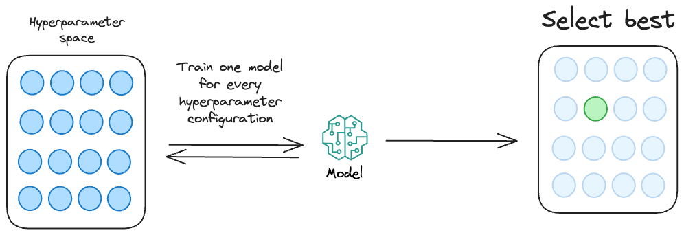
While this approach is feasible for training small-scale ML models, it is practically infeasible when training bigger models.

To get some perspective, imagine if it takes $1.5$ hours to train a model and you have set $20$ different hyperparameter configurations to run through your model.

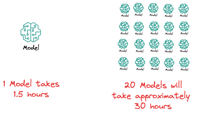
That's more than a day of training.

Therefore, learning about optimized hyperparameter tuning strategies and utilizing them is extremely important to build large ML models.

Bayesian optimization is one such immensely powerful approach for tuning hyperparameters.

The idea is that while iterating over different hyperparameter configurations, the Bayesian optimization algorithm constantly updates its beliefs about the distribution of hyperparameters by observing model performance corresponding to each hyperparameter.

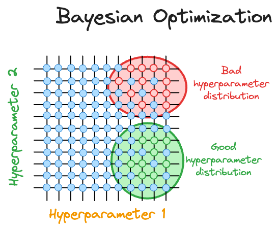
This allows it to take informed steps to select the next set of hyperparameters, gradually converging to an optimal set of hyperparameters.

To understand better, consider that we have the following results with grid search:

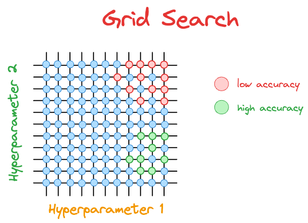
The hyperparameter configurations with low accuracy are marked in red, and those with high accuracy are marked in green.

After the $21$ model runs ($9$ green and $12$ red) depicted above, the grid search will not make any informed guesses on which hyperparameter it should evaluate next.

In other words, all trials operate independently.

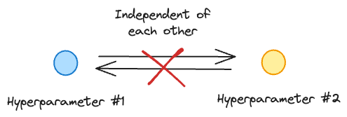
But if we look at the evaluation results in the figure below, doesn't it make more sense to concentrate our hyperparameter search near the green region?

That is the core idea behind Bayesian optimization.

Simply put, Bayesian optimization works as follows:

• Build a probability model of the objective function, which is conditioned on the hyperparameter. The objective function can be loss or accuracy.
• Use the probability model to make informed decisions about the most promising hyperparameters.

Thus, it uses past results to form a probabilistic model, which maps the hyperparameters to a probability of achieving a score using the objective function: