HDBSCAN: The Supercharged Version of DBSCAN — An Algorithmic Deep Dive

We have covered quite a few advanced clustering algorithms before here, like the following:

Gaussian Mixture Models (GMMs)

Gaussian Mixture Models: A more robust alternative to KMeans.

Daily Dose of Data ScienceAvi Chawla

DBSCAN++: The Faster and Scalable Alternative to DBSCAN Clustering

Addressing major limitations of the most popular density-based clustering algorithm — DBSCAN.

Daily Dose of Data ScienceAvi Chawla

In this article, let's continue the clustering series and cover HDBSCAN, a powerful hierarchical clustering algorithm that extends the capabilities of DBSCAN by adding hierarchical clustering and handling varying densities more effectively.

• DBSCAN stands for Density-Based Spatial Clustering of Applications with Noise.
• HDBSCAN stands for Hierarchical Density-Based Spatial Clustering of Applications with Noise.

We covered it briefly in the newsletter as well recently:

HDBSCAN vs. DBSCAN

What limitations does HDBSCAN address?

Daily Dose of Data ScienceAvi Chawla

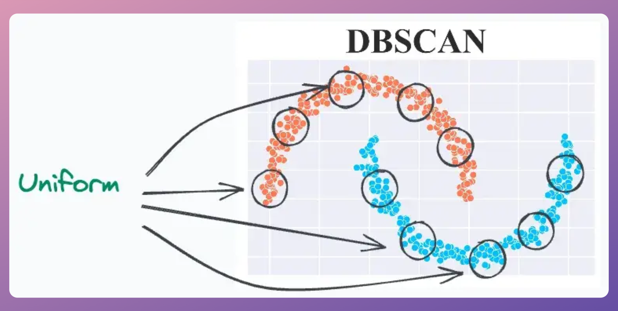
To reiterate, DBSCAN assumes that the local density of data points is (somewhat) globally uniform. This is governed by its eps parameter.

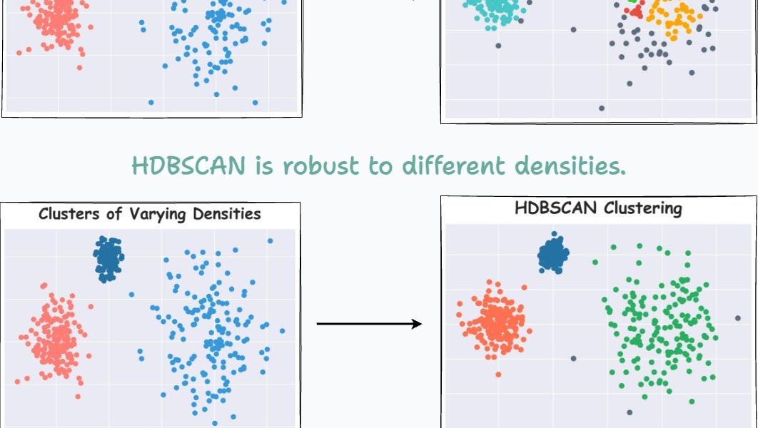
For instance, consider the clustering results obtained with DBSCAN on the dummy dataset below, where each cluster has different densities:

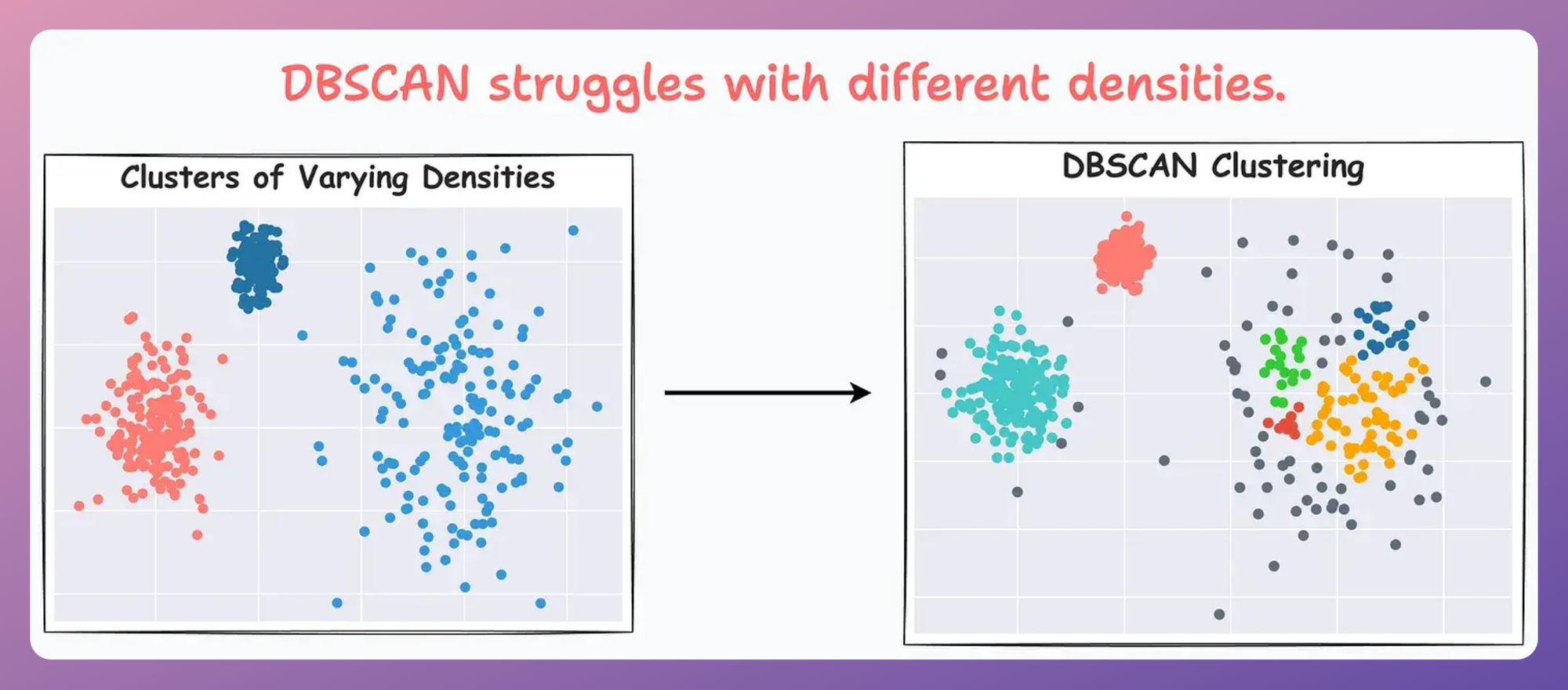
It is clear that DBSCAN produces bad clustering results.

Now compare it with HDBSCAN results depicted below:

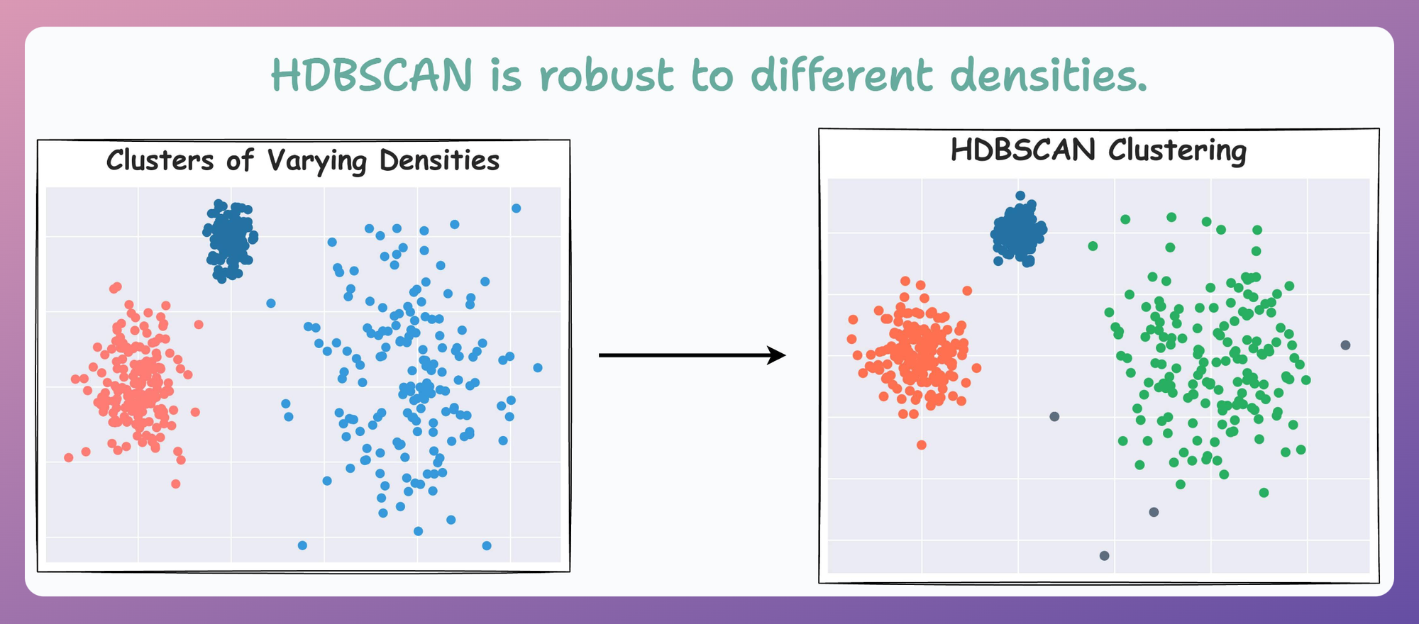
On a dataset with three clusters, each with varying densities, HDBSCAN is found to be more robust.

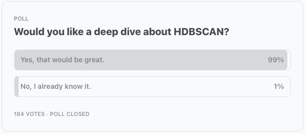
Towards the end, most readers also showed interest in a deep dive into HDBSCAN, so it appears to be a great topic to cover.

In this article, we shall cover the key concepts that will help you understand how HDBSCAN works and why it is a powerful clustering algorithm.

Let's begin!

What’s the data like?

Any clustering dataset begins with some dataset (unlabeled) and a few assumptions about it.

Before devising (or utilizing) any clustering algorithm, the first question we need to answer is:

What do we know about the given data? What type of data are we trying to cluster?

Ideally, we would want to make as few assumptions so two core assumptions that we can proceed with are:

• The dataset has noise, which means that not every point will belong to a cluster.
• There are some clusters (we don't know how many) of arbitrary shapes in the given dataset.

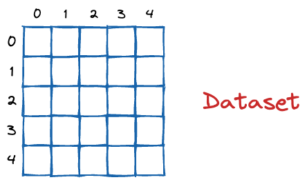
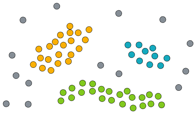
In this article, we shall focus and build the foundations for HDBSCAN clustering using the following 2D dataset:

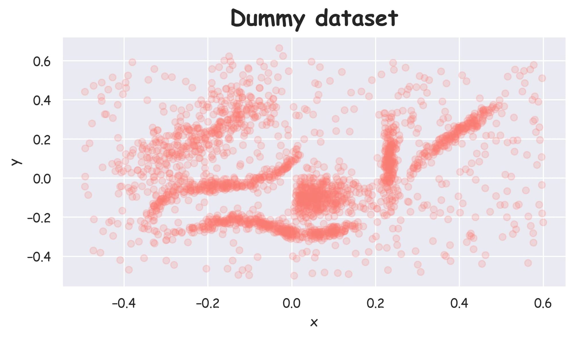
Being a 2D dataset, it's pretty easy to visually assess that there are 6 clusters in this dataset, and others are noise points:

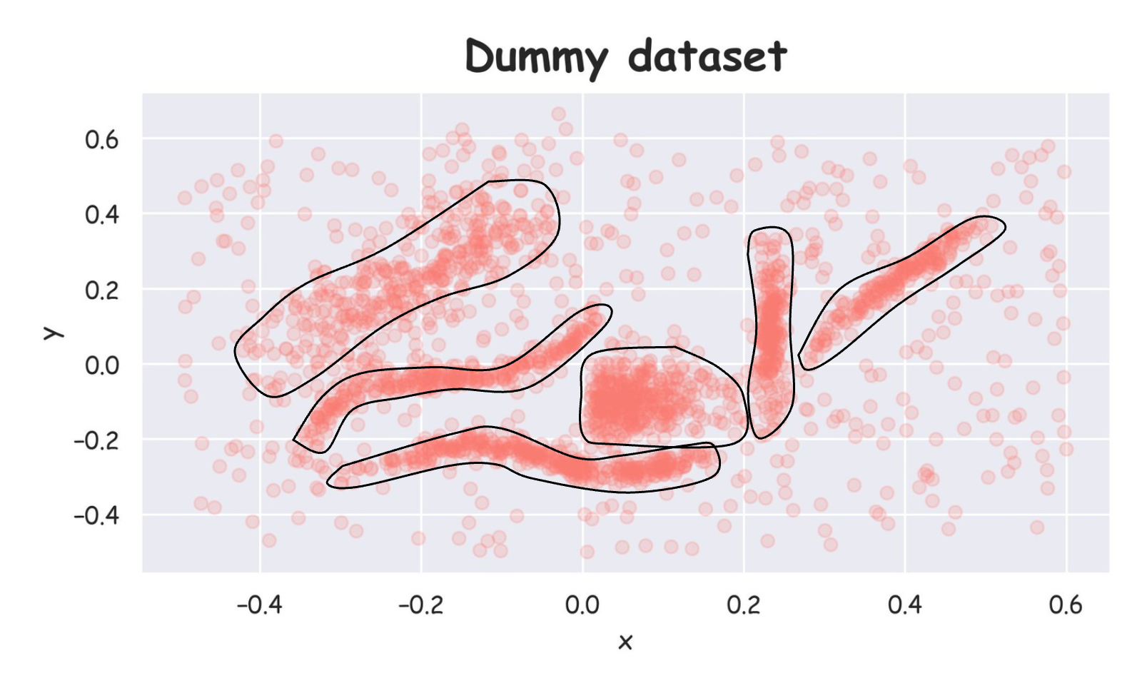
But of course, visual methods are not feasible in all cases (especially high-dimensional datasets), so we expect to have a clustering algorithm that can identify clusters for us in any high-dimensional space.

Using KMeans

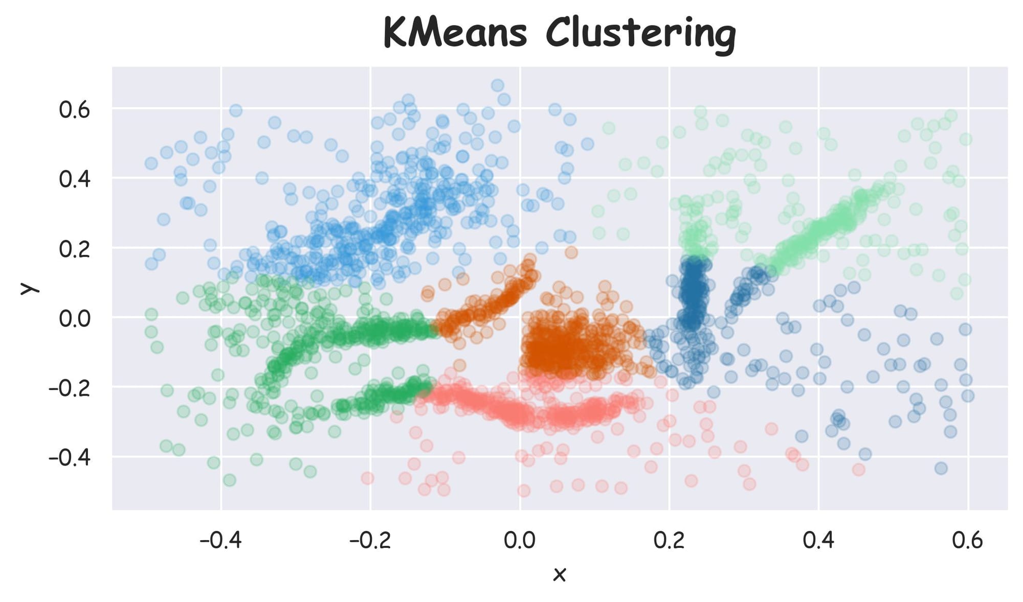
One of the first instincts in all clustering is to try KMeans. As the number of clusters is known to us in this specific instance, let's run KMeans clustering and plot the results:

Plotting the dataset with clustering labels (labels), we get the following plot:

For a moment, let’s just assume that we already have an implementation for the HDBSCAN algorithm and we run it on the above dataset:

Plotting the dataset with clustering labels (labels), we get the following plot:

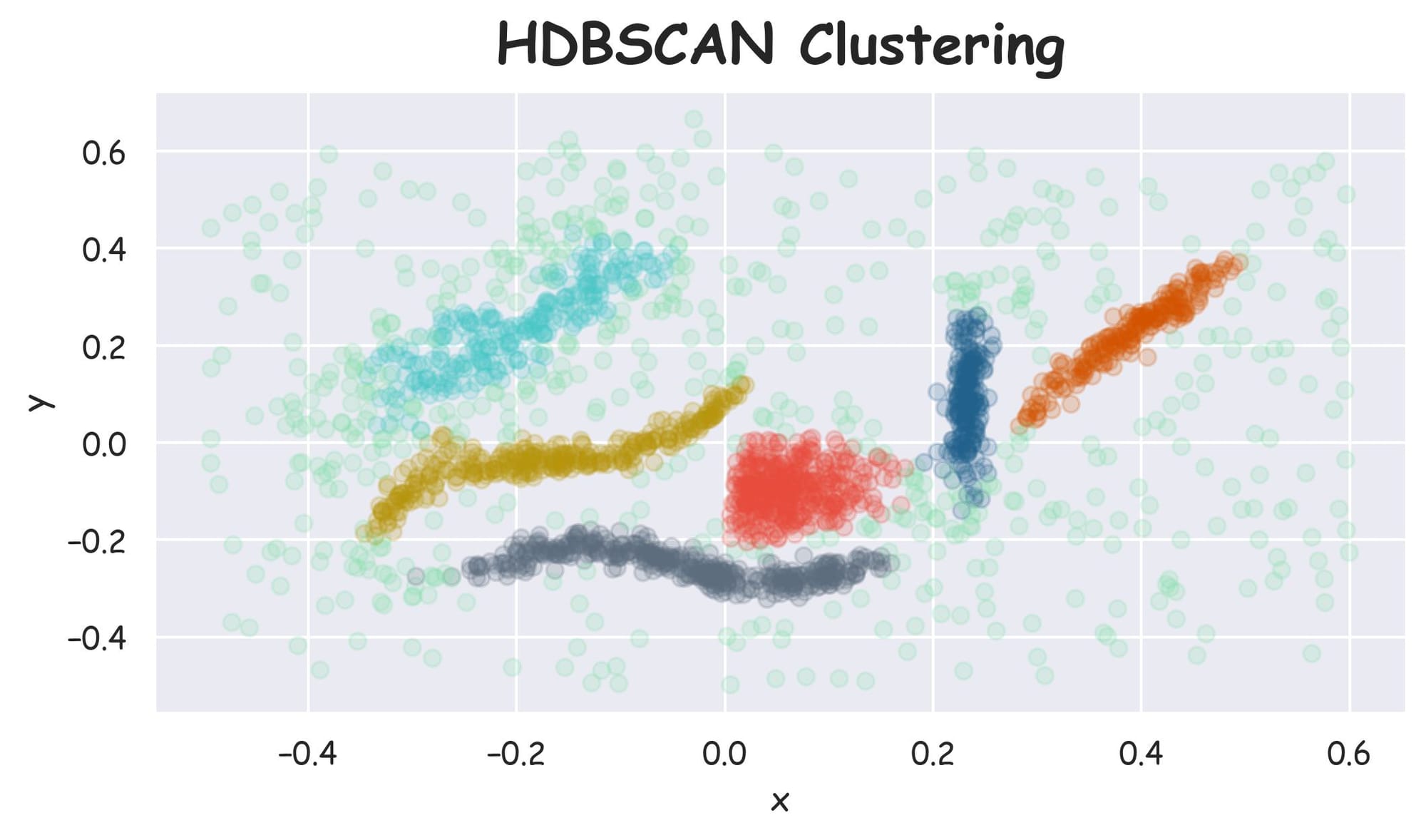
Despite specifying the number of clusters in KMeans, it failed to cluster the dataset into appropriate clusters. However, HDBSCAN did a better clustering (based on visual assessment) without specifying the number of clusters.

Why did KMeans fail?

Let's understand!

Limitations of KMeans

While its simplicity often makes it the most preferred clustering algorithm, KMeans has many limitations that hinder its effectiveness in many scenarios.

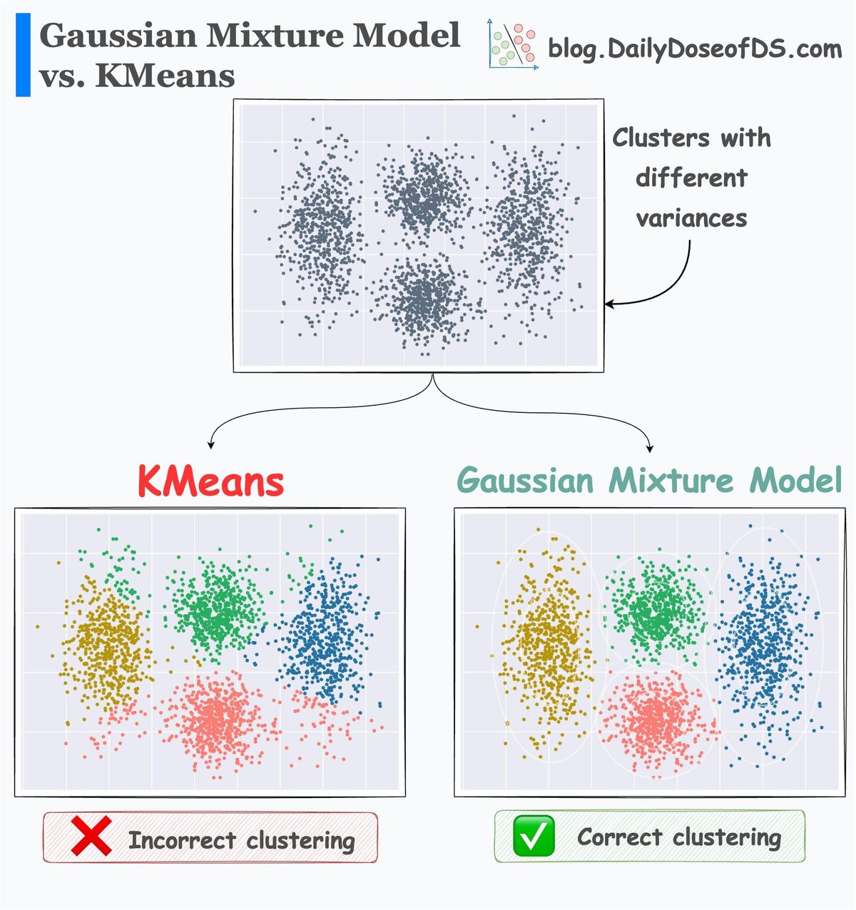
#1) KMeans does not account for cluster variance and shape

For instance, KMeans does not account for cluster variance and shape.

In other words, one of the primary limitations of KMeans is its assumption of spherical clusters.

One intuitive and graphical way to understand the KMeans algorithm is to place a circle at the center of each cluster, which encloses the points.

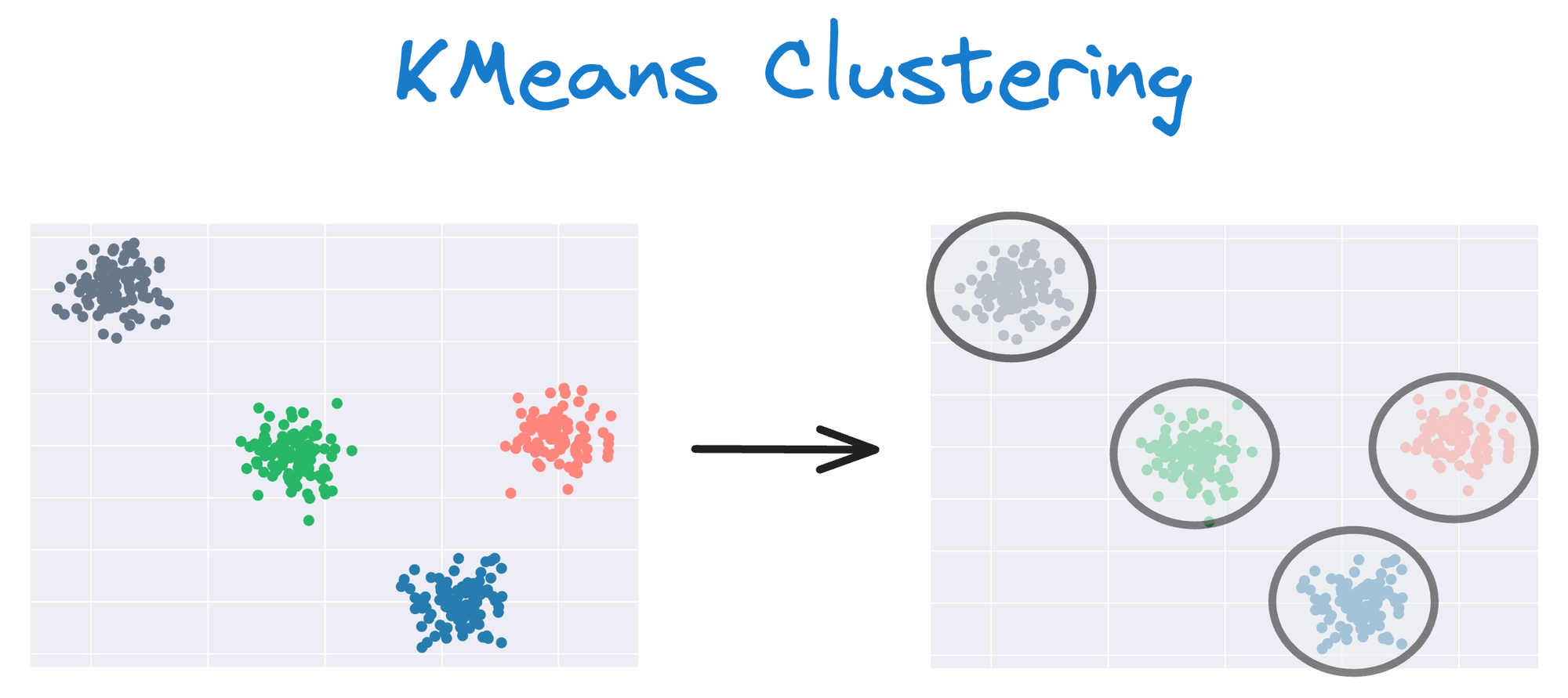
As KMeans is all about placing circles, its results aren’t ideal when the dataset has irregular shapes or varying sizes, as shown below:

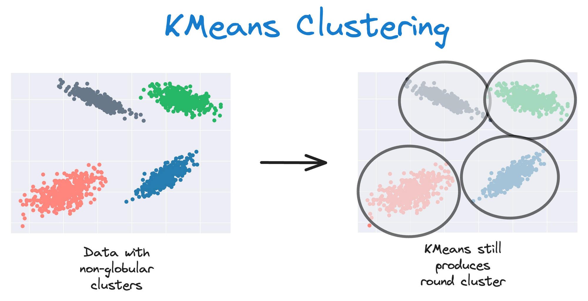
Instead, an ideal clustering should cluster the data as follows:

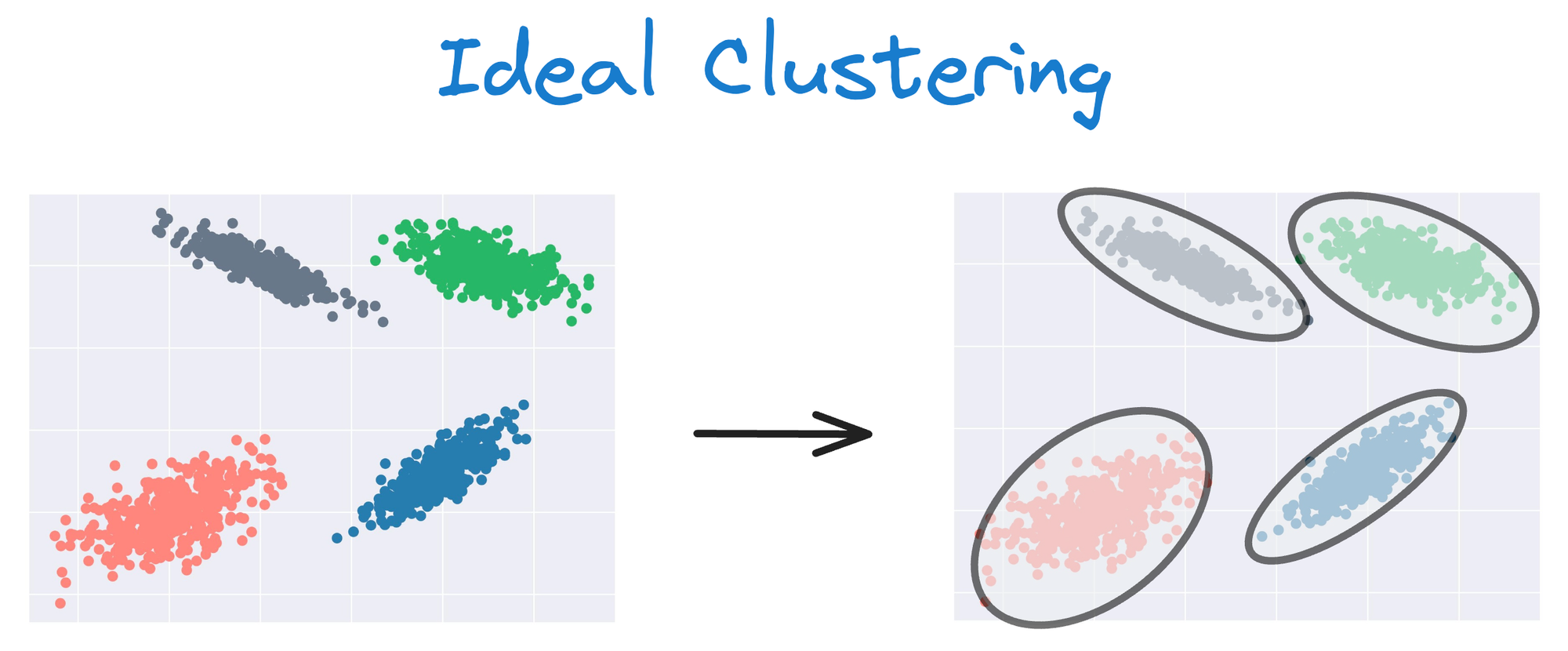
The same can be observed in the following dataset:

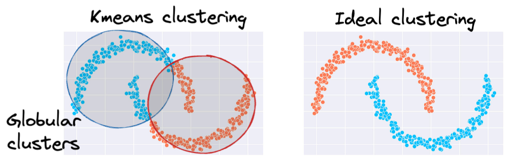
This rigidity of KMeans to only cluster globular clusters often leads to misclassification and suboptimal cluster assignments.

#2) Every data point is assigned to a cluster

Another significant limitation of the KMeans clustering algorithm is its inherent assumption that every data point must be assigned to a cluster.