DBSCAN++: The Faster and Scalable Alternative to DBSCAN Clustering
Addressing major limitations of the most popular density-based clustering algorithm — DBSCAN.
Introduction
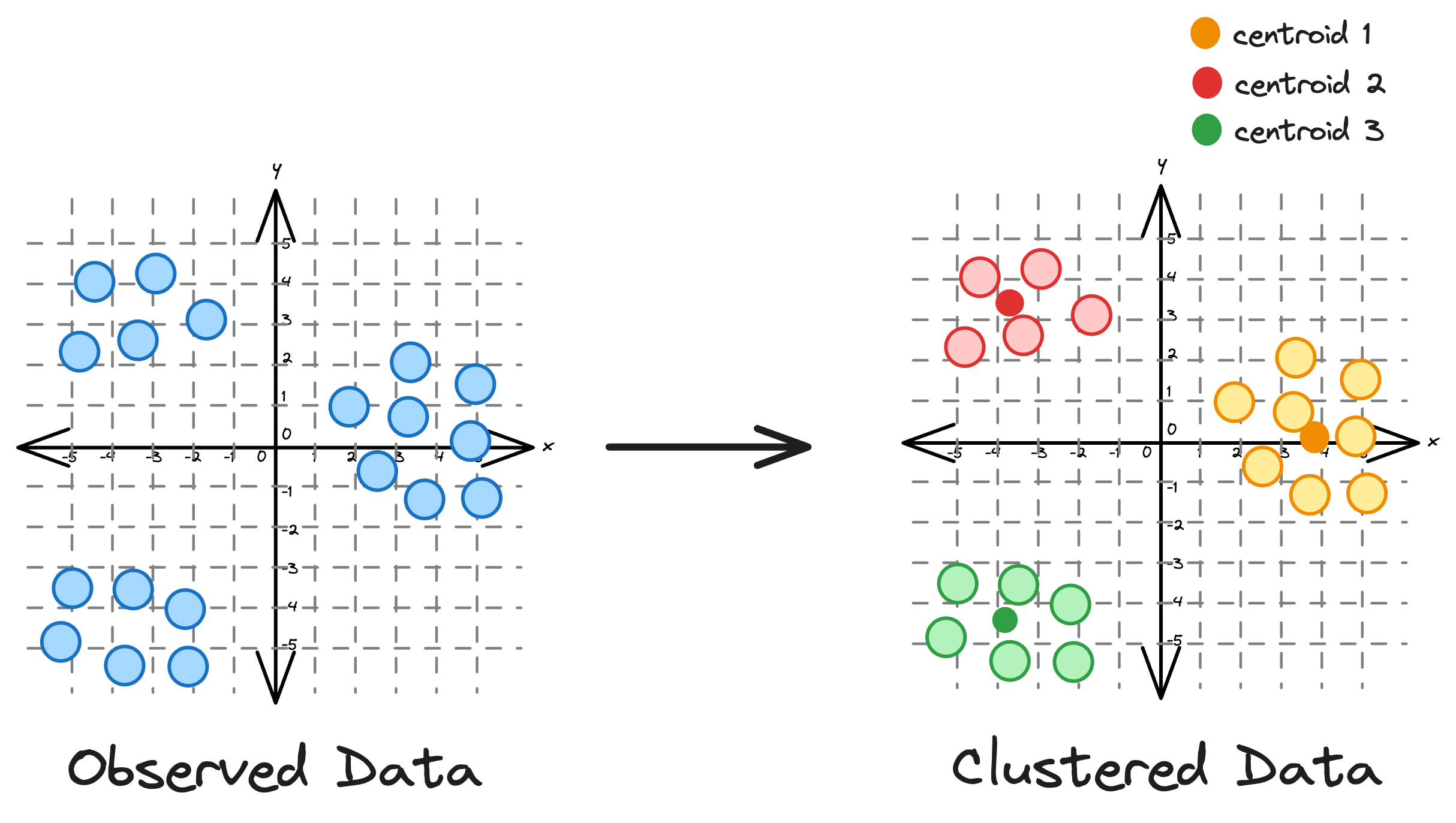
KMeans is an unsupervised clustering algorithm that groups data based on distances. It is widely recognized for its simplicity and effectiveness as a clustering algorithm.
Essentially, the core idea is to partition a dataset into distinct clusters, with each point belonging to the cluster whose centroid is closest to it.
Limitations of KMeans
While its simplicity often makes it the most preferred clustering algorithm, KMeans has many limitations that hinder its effectiveness in many scenarios.
#1) KMeans does not account for cluster variance and shape
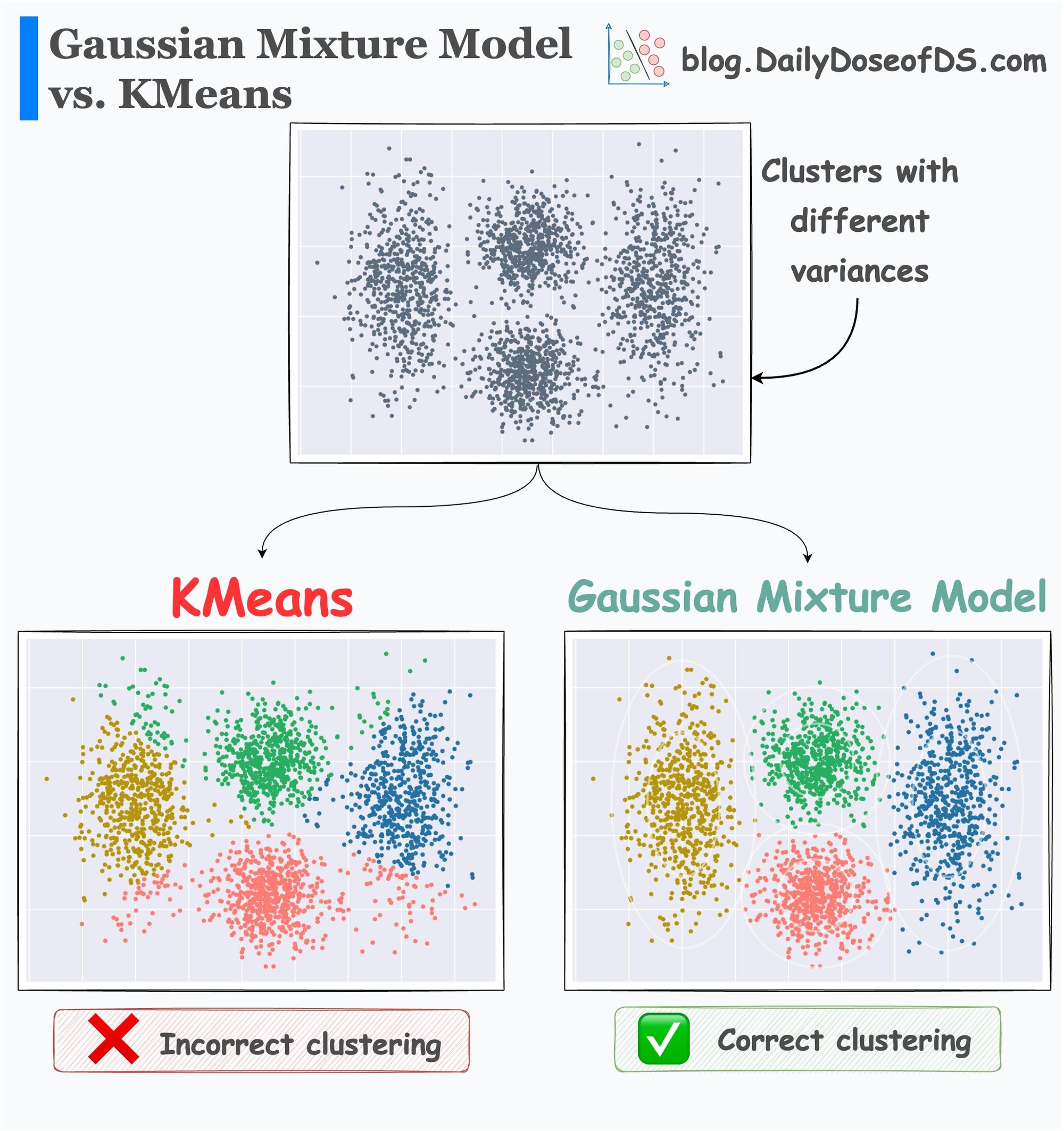
For instance, KMeans does not account for cluster variance and shape.
In other words, one of the primary limitations of KMeans is its assumption of spherical clusters.
One intuitive and graphical way to understand the KMeans algorithm is to place a circle at the center of each cluster, which encloses the points.
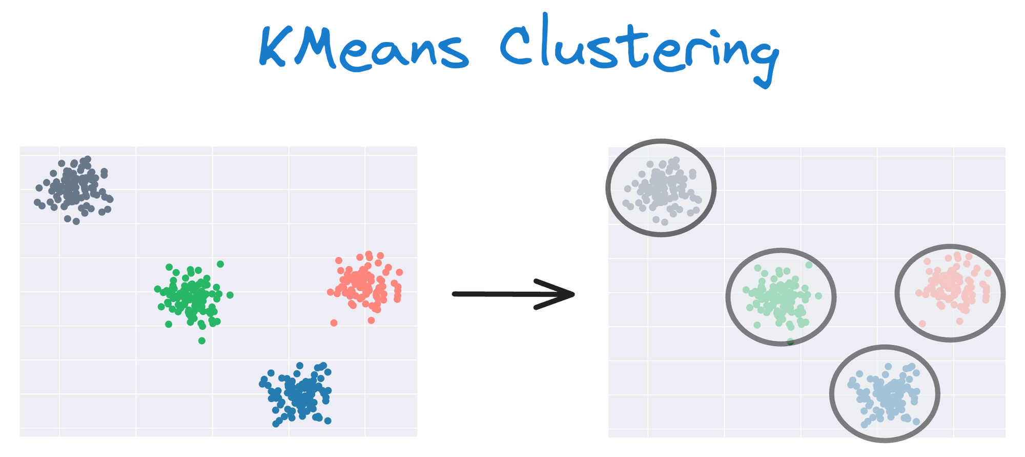
As KMeans is all about placing circles, its results aren’t ideal when the dataset has irregular shapes or varying sizes, as shown below:
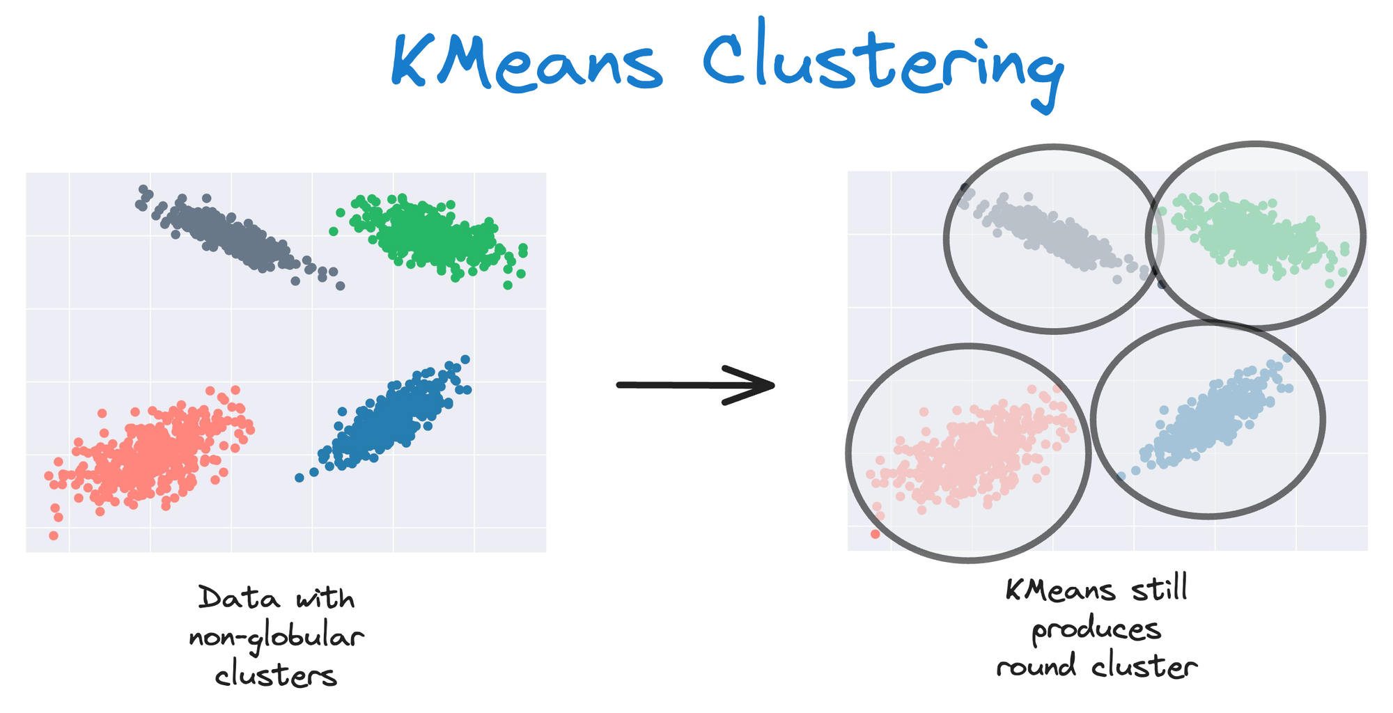
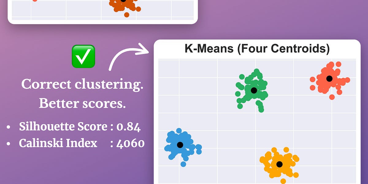
Instead, an ideal clustering should cluster the data as follows:
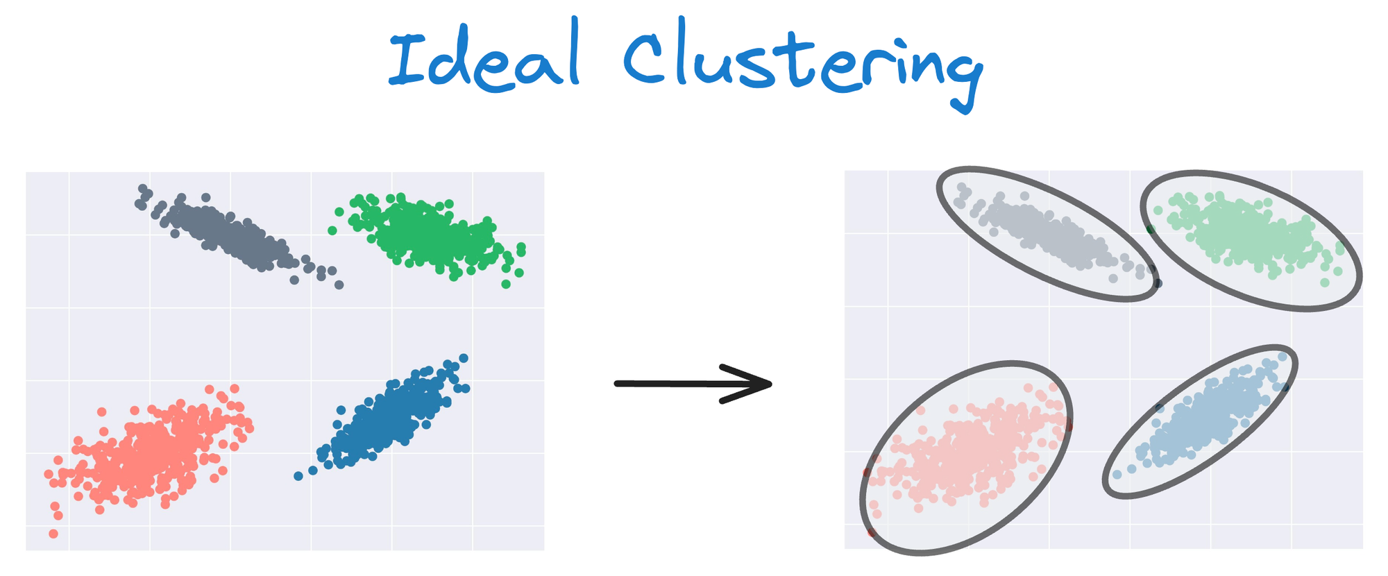
The same can be observed in the following dataset:

This rigidity of KMeans to only cluster globular clusters often leads to misclassification and suboptimal cluster assignments.
#2) Every data point is assigned to a cluster
Another significant limitation of the KMeans clustering algorithm is its inherent assumption that every data point must be assigned to a cluster.
More specifically, KMeans operates under the premise that each data point belongs to one and only one cluster, leaving no room for the representation of noise or outliers.
This characteristic can be problematic in scenarios where the dataset contains irregularities, anomalies, or noise that do not conform to clear cluster boundaries.
As a result, KMeans may inadvertently assign data points to clusters even when they do not truly belong to any discernible pattern.
This is depicted in the image below:
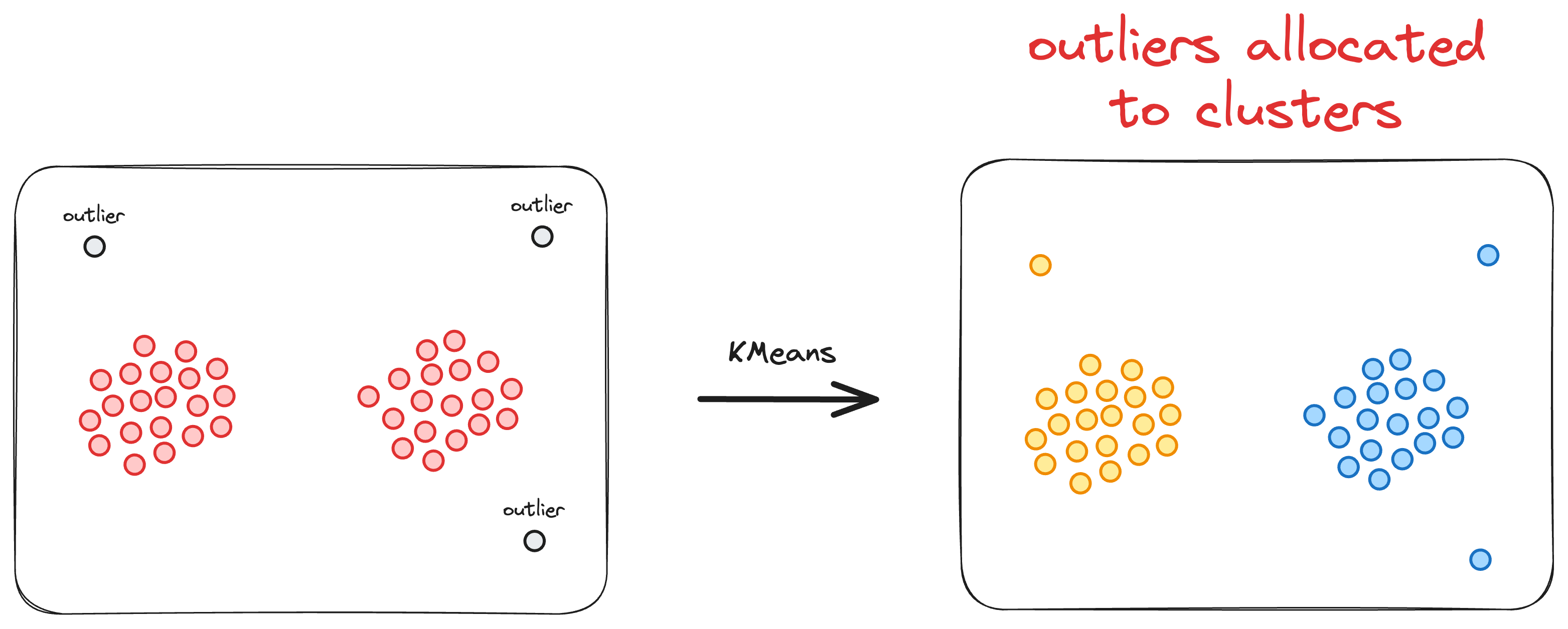
This tendency can lead to suboptimal clustering results, particularly in datasets with varying densities, irregular shapes, or the presence of noisy data.
In real-world datasets where the underlying structure is not well-suited to the assumptions of KMeans, the algorithm’s rigid assignment of all data points to clusters can limit its effectiveness.
We should be mindful of this limitation and consider alternative clustering approaches, such as density-based or hierarchical methods, when dealing with datasets that exhibit significant noise or outliers.
#3) Specification of the number of clusters
One notable constraint of using the K-Means clustering algorithm is the requirement for prior knowledge or assumptions about the exact number of clusters in the dataset.
Unlike some other clustering algorithms that can automatically determine the optimal number of clusters based on the data's inherent structure, K-Means relies on a predefined value for the number of clusters (often denoted as 'k').
Of course, this is not a problem though, and there are various methods to determine a reliable value for the parameter $k$, but that constraint poses challenges in scenarios where the true number of clusters is not known in advance, leading to potential inaccuracies and suboptimal results.
On a side note, we commonly use the Elbow curve to determine the number of clusters (k) for KMeans.
However, the problem with the Elbow curve is that it:
- has a subjective interpretation
- involves ambiguity in determining the Elbow point accurately
- only considers a within-cluster distance, and more.
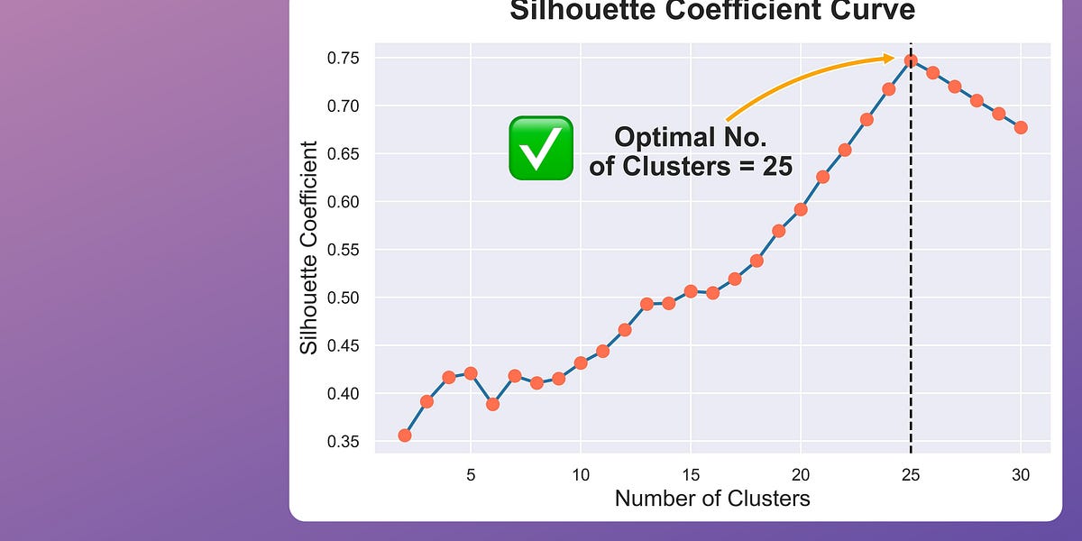
Silhouette score is an alternative measure used to evaluate clustering quality, and it is typically found to be more reliable than the Elbow curve.
Measuring it across a range of centroids (k) can reveal which clustering results are most promising.
The visual below compares the Elbow curve and the Silhouette plot:
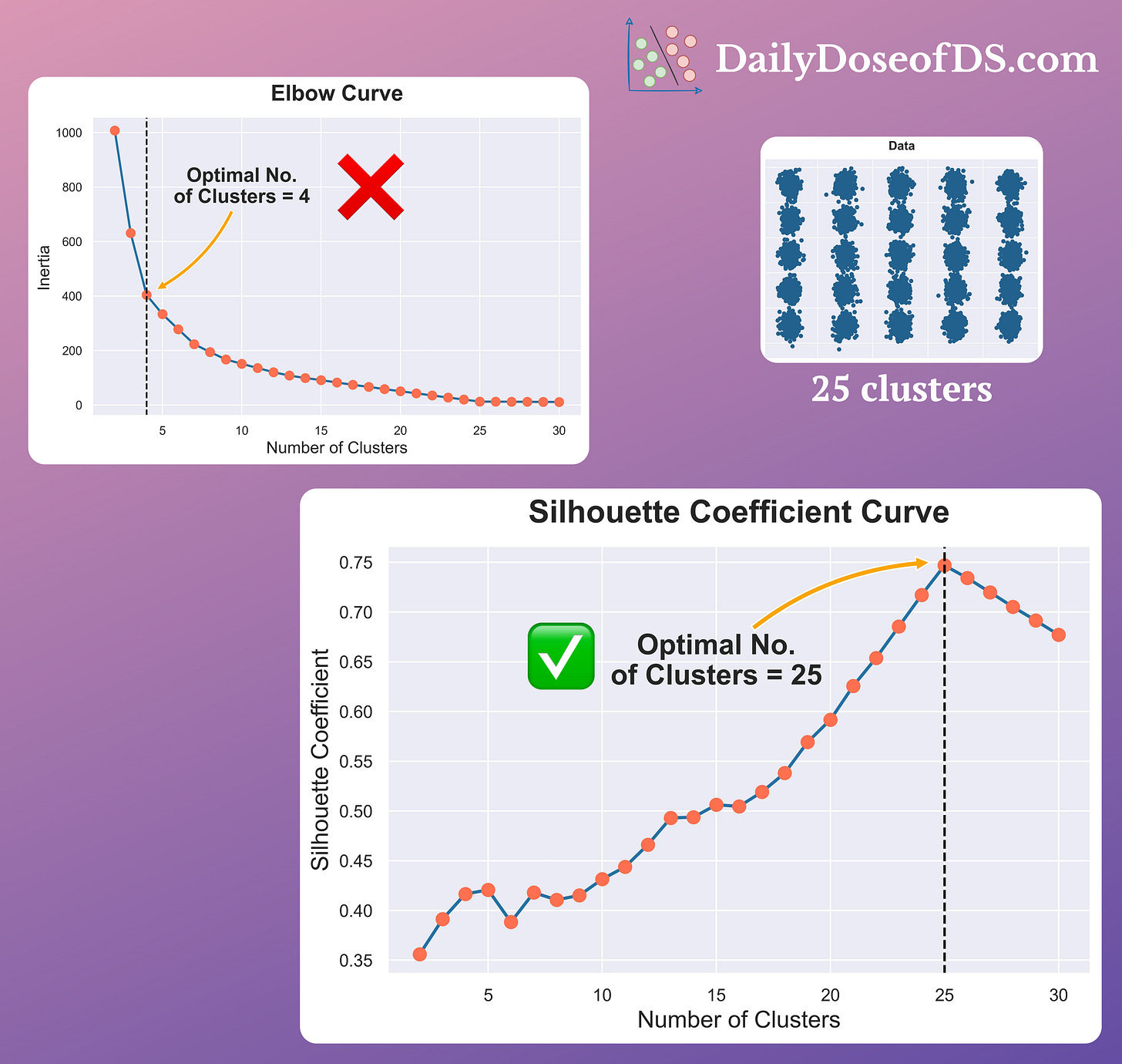
It’s clear that the Elbow curve is highly misleading and inaccurate.
In a dataset with 25 clusters:
- The Elbow curve depicts four as the number of optimal clusters.
- The Silhouette curve depicts 25 as the number of optimal clusters.
We have already covered this in a couple of previous newsletter issues if you want to get into more details:
Coming back...
The above limitations of KMeans highlight the importance of learning about other better algorithms that we can use to address these limitations is extremely important.
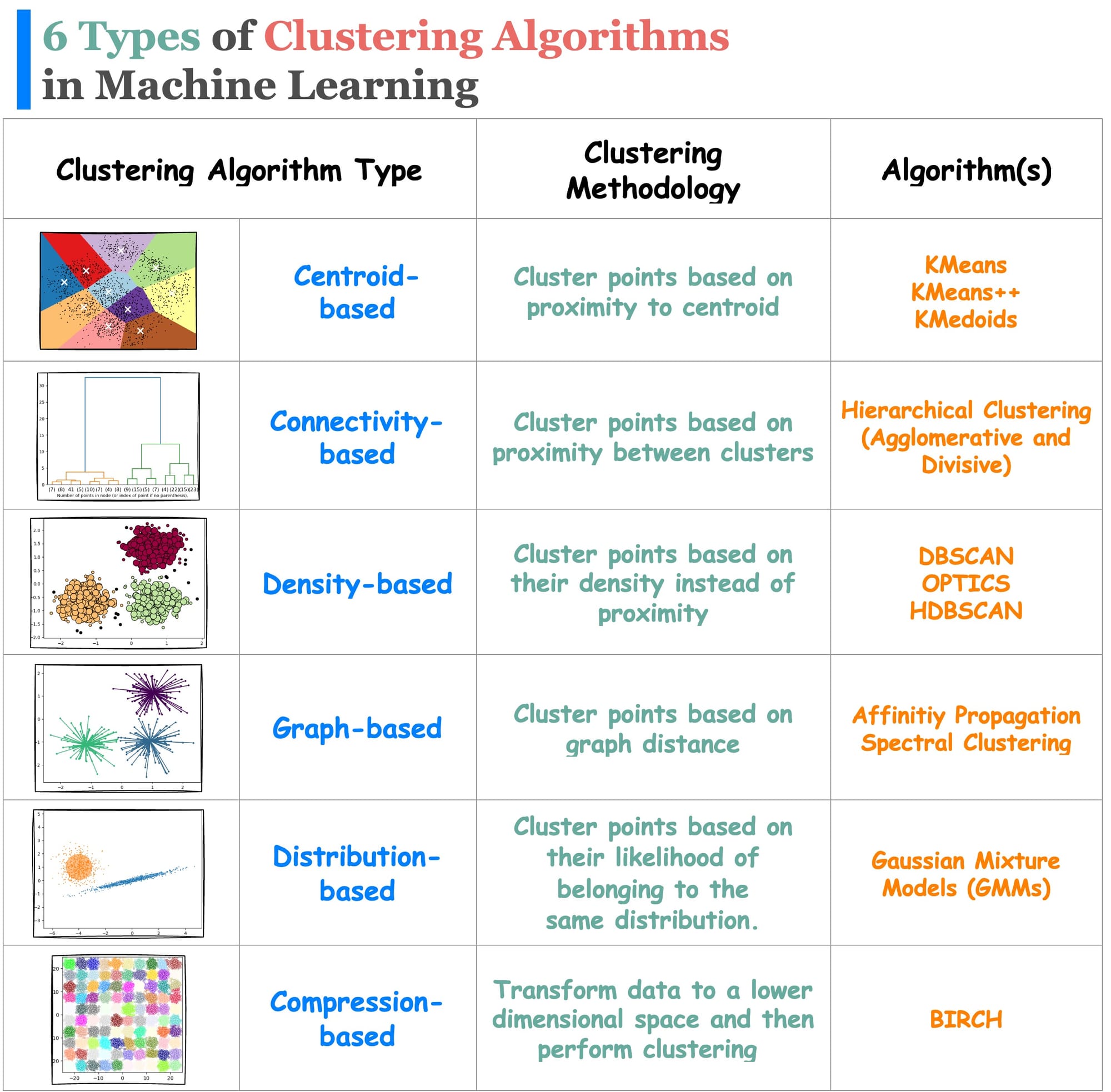
While KMeans comes under the centroid-based clustering algorithms, there are many different types of clustering algorithms (shown below) that can be used depending on the situation:
We have already covered distribution-based clustering before:
So the focus of this article is Density-based clustering, that too specifically DBSCAN++, which is a significant improvement on the DBSCAN clustering algorithm.
Let’s understand in detail!
But before understanding DBSCAN++, let’s understand what DBSCAN is.
What is DBSCAN?
DBSCAN, which stands for Density-Based Spatial Clustering of Applications with Noise, is a popular clustering algorithm in machine learning and data mining.
As the name suggests, the core idea behind DBSCAN is to group together data points based on “density”, i.e., points that are close to each other in a high-density region and are separated by lower-density regions.

It does a great job of seeking areas in the data with a high density of data points, versus areas of the data that are not very dense with observations.
The notion of density in DBSCAN lets it sort data into clusters of varying shapes as well, which is its substantial advantage over traditional clustering algorithms such as KMeans.
As a result, it immediately resolves each of the above-discussed limitations of the KMeans clustering algorithm.
- As it clusters based on the notion of “density”, the clusters may not necessarily have a globular shape. Instead, they may have arbitrary shapes, as depicted below:

- Unlike KMeans, DBSCAN does not allocate each data point to a cluster. This is because DBSCAN operates on a fundamentally different principle—density-based clustering. Outliers are regions of very low density, and we will see shortly that DBSCAN can quickly identify regions of low density and classify points in those regions as outliers.
- What’s more, another benefit of DBSCAN is that it doesn’t require specifying the number of clusters in advance. Instead, it identifies clusters based on the density of data points.
How it works?
We will walk through a simple example to understand how the algorithm works.
Let’s say we have a dataset of points like the following:
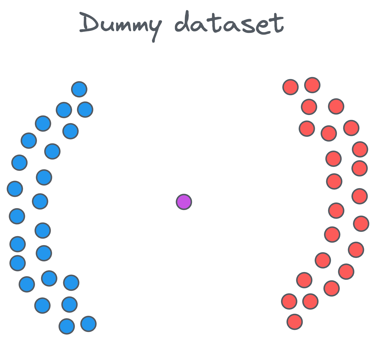
Clearly, we have two distinct clusters and one noise point at the center. Our objective is to cluster these points into groups that are densely packed together.
Firstly, we count the number of points in the vicinity of each data point. For example, if we start with the green point, we draw a circle around it.
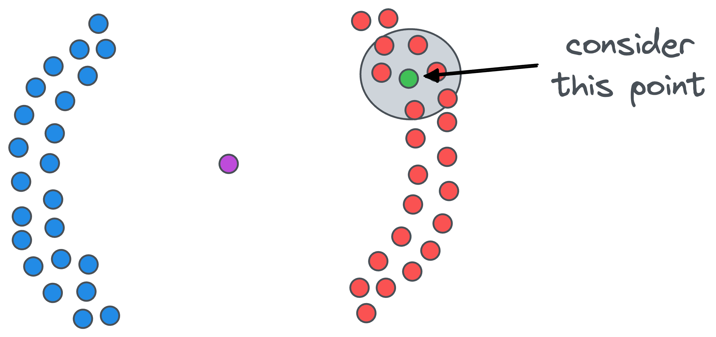
The radius epsilon of the circle is the first parameter that we must specify when using DBSCAN. In other words, this is a hyperparameter.

After drawing the circle, we count the number of data points that fall within that $\epsilon$ radius circle. For instance, for our green point, there are six close points.
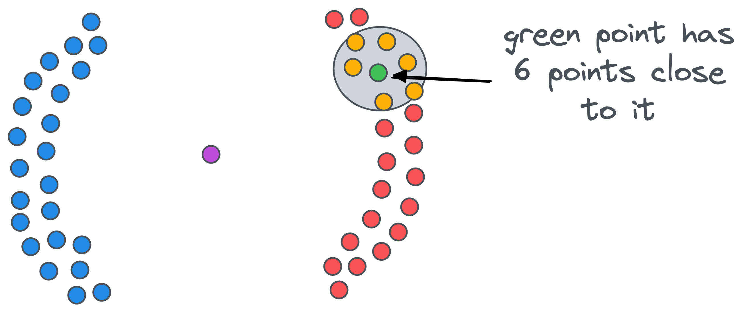
Likewise, we count the number of close points for all remaining points.
After counting the number of data points in the vicinity of each data point, we classify every data point into one of the three categories:
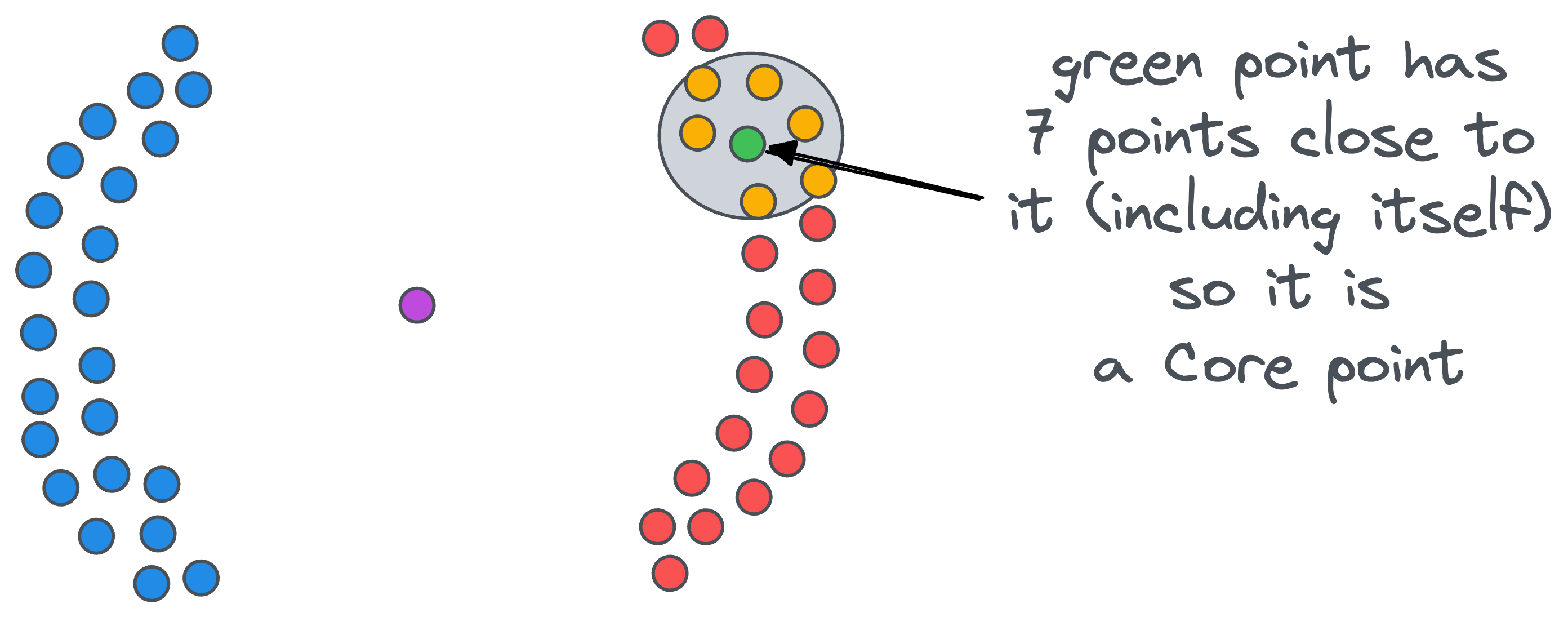
- Core point: A data point that has at least
minPtsdata points (including the point itself) at a distance less than equal toepsilon. For instance, ifminPts=5, the green point in the figure below is a core point:
- Border point: A data point that does not have at least
minPtsdata points (including the point itself) at a distance less than equal toepsilon, but it is in the vicinity of a core point. For instance, in the figure below, the green point is a border point.
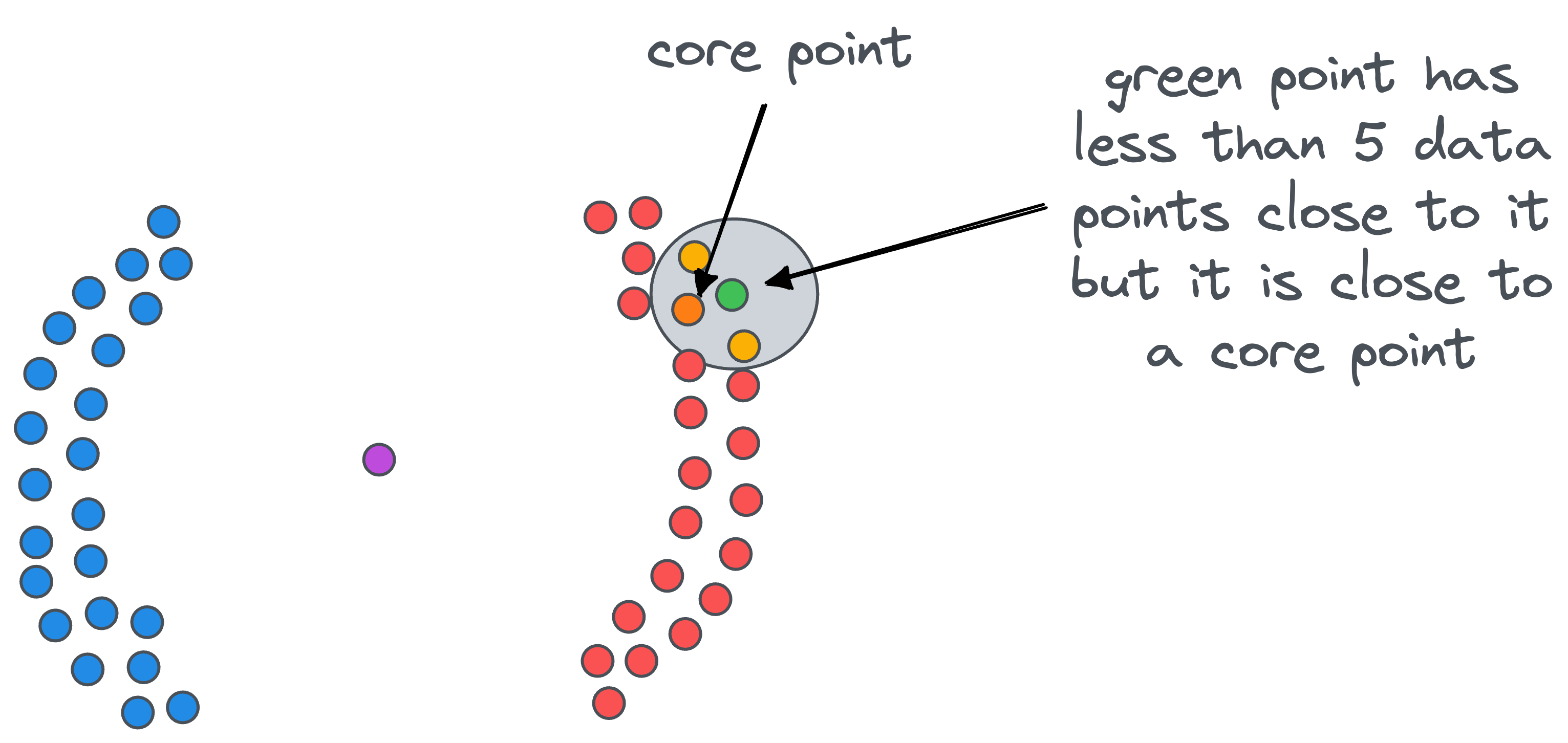
- Noise point: A data point that is neither a core point nor a border point is a noise point. For instance, in the figure below, the purple data point is a noise point:
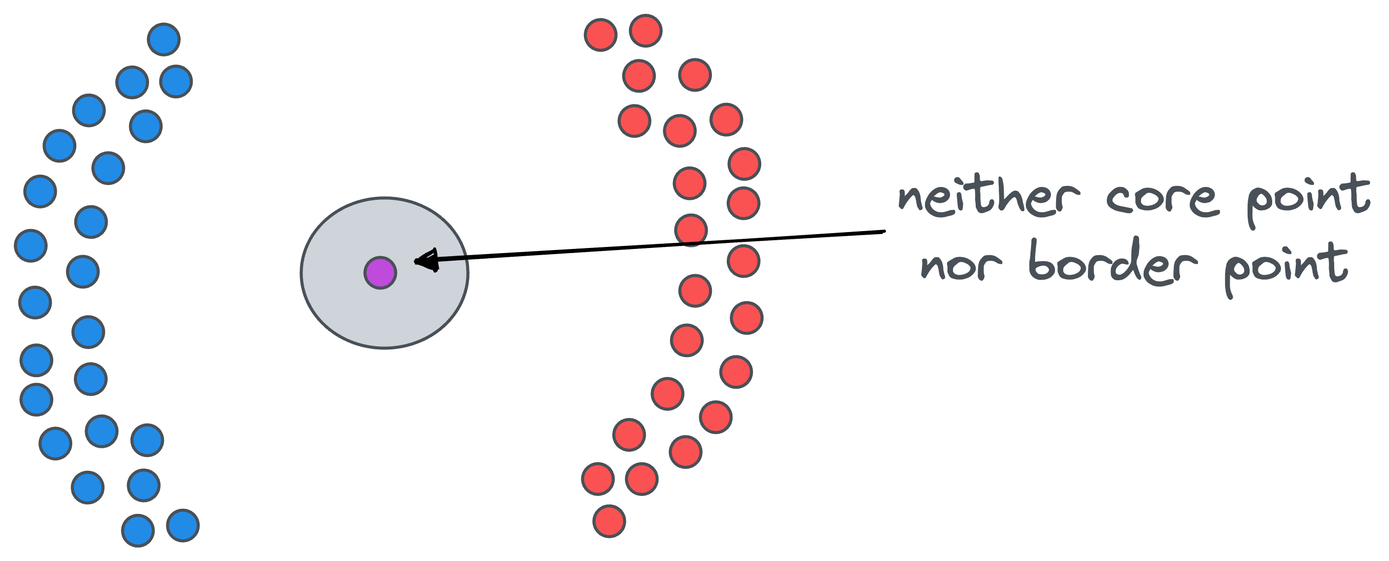
And of course, as you may have already guessed, minPts is another hyperparameter of DBSCAN.
After classifying all the data points as core, border, or noise points, we proceed with clustering.
The idea is simple.
- Start with any core point (let’s call it
A) and assign it to a cluster with cluster-ID, say1(to begin).
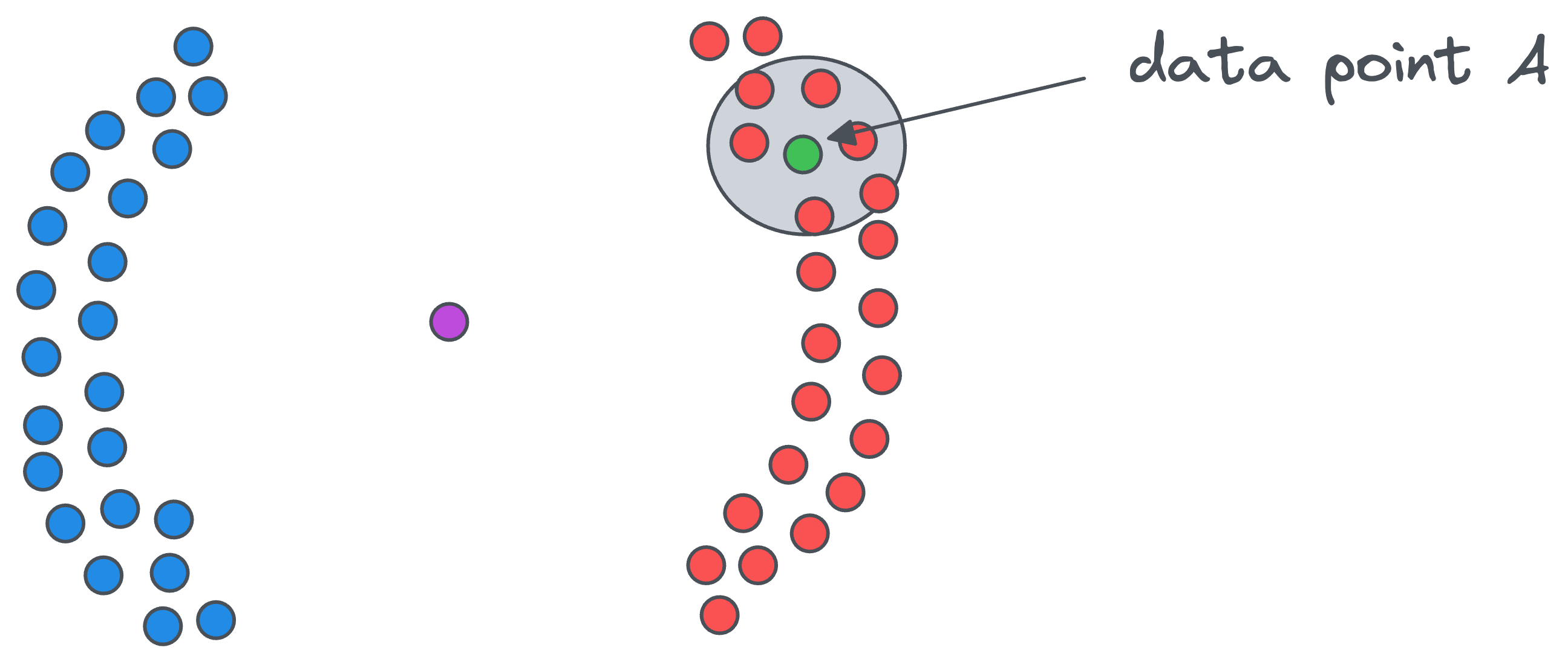
- All points in the vicinity of the above core point
Awill belong to the same cluster — whose cluster-ID is1.
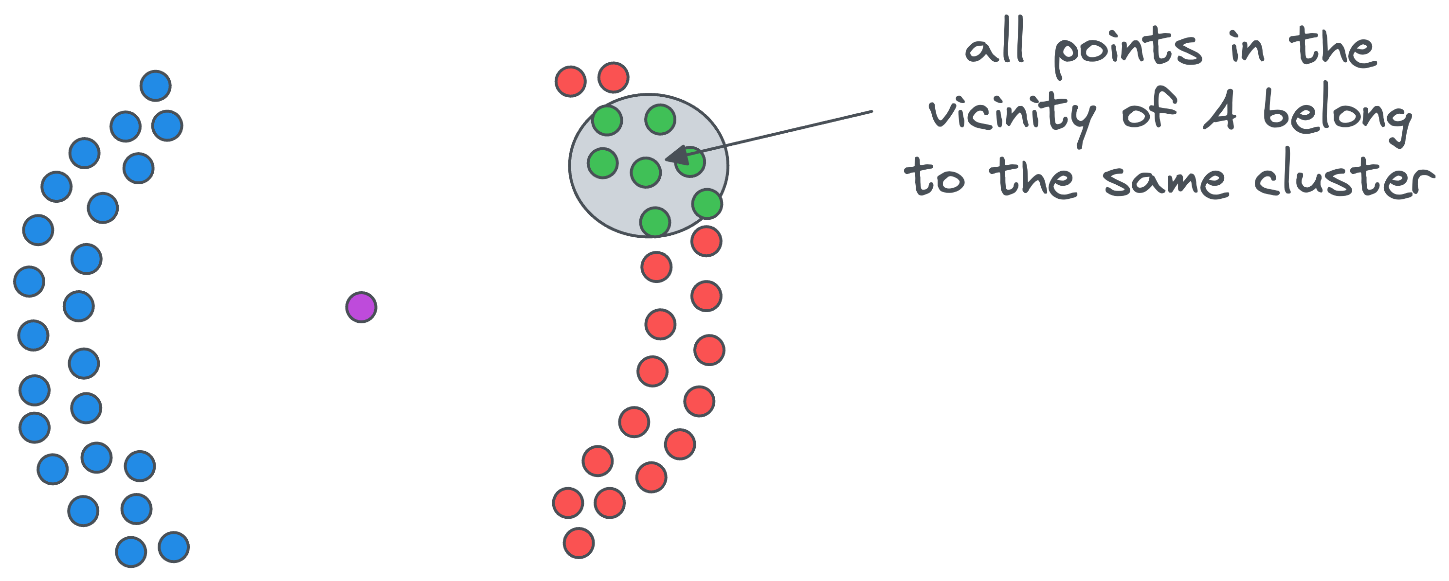
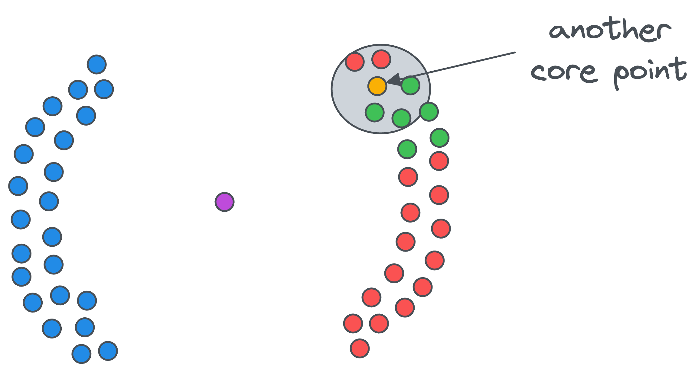
- If a data point in the vicinity of the core point
Ais also a core point, as shown below...
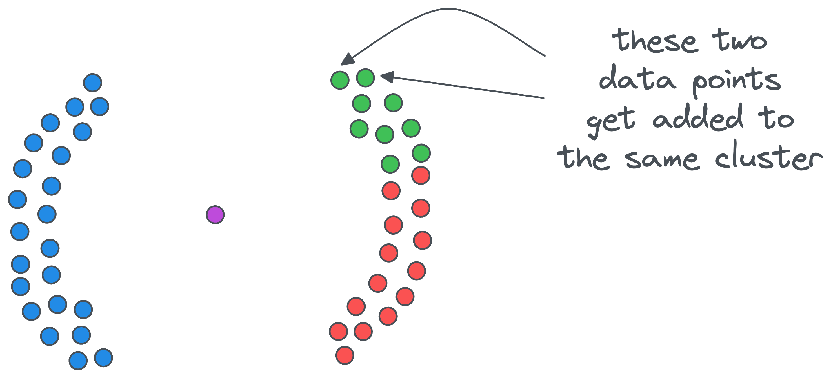
- ....then we include data points in its vicinity in the same cluster — whose cluster ID is
1.
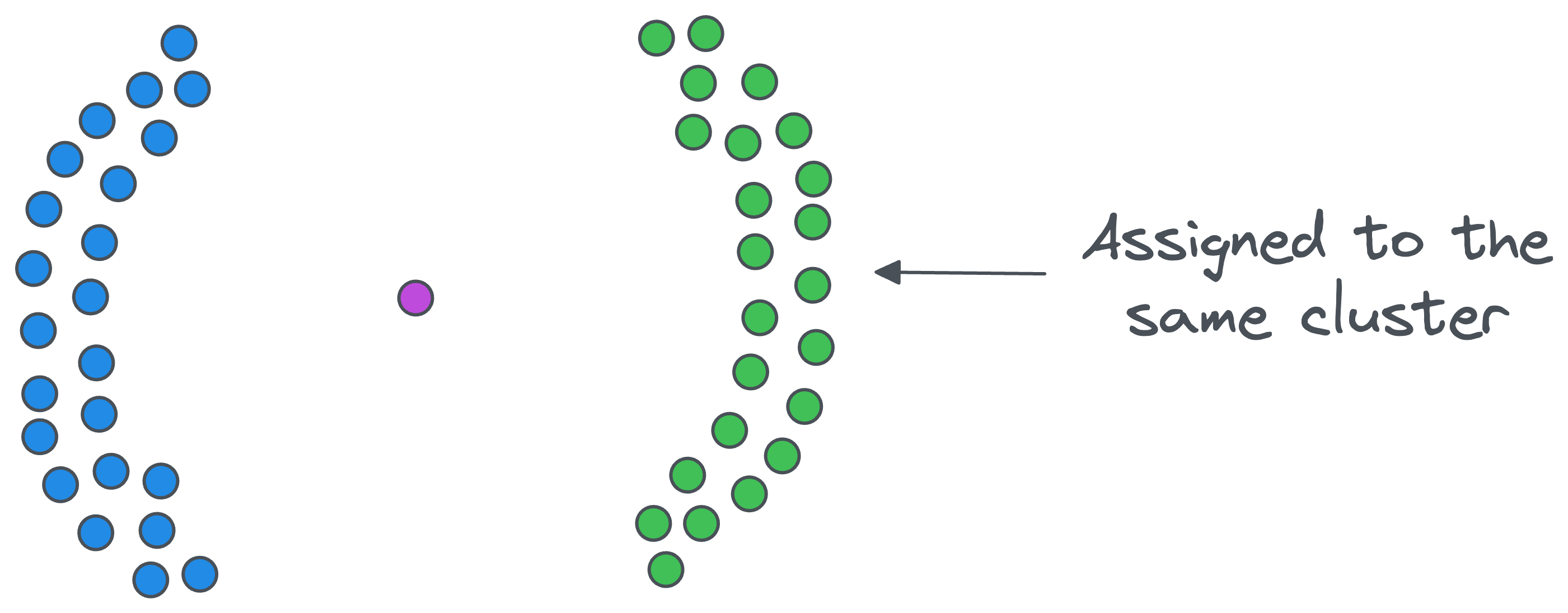
- The above step is executed recursively under the same cluster-ID until we cannot find a new core point.
- At this point, we may still have some core points in the dataset, but they may not belong to the previous cluster, as shown below. We repeat the same steps as above but with a new cluster ID this time.
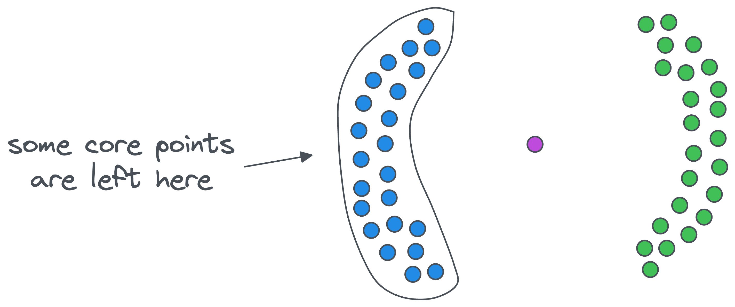
The algorithm completes its execution once we are left with no core points.
How to Find Optimal Epsilon Value
In DBSCAN, determining the epsilon parameter is often tricky. But the Elbow curve is often helpful in determining it.
To begin, as we discussed above, DBSCAN has two hyperparameters:
epsilon: two points are considered neighbors if they are closer than Epsilon.minPts: Min neighbors for a point to be classified as a core point.
We can use the Elbow curve to find an optimal value of epsilon:
For every data point, plot the distance to its $k^{th}$ nearest neighbor (in increasing order), where k is the minPts hyperparameter. This is called the k-distance plot.
The optimal value of epsilon is found near the elbow point.
Why does it work?
Recall that in this plot, we are measuring the distance to a specific ($k^{th}$) neighbor for all points. Thus, the elbow point suggests a distance to a more isolated point or a point in a different cluster.
The point where change is most pronounced hints towards an optimal epsilon. The efficacy is evident from the image above.
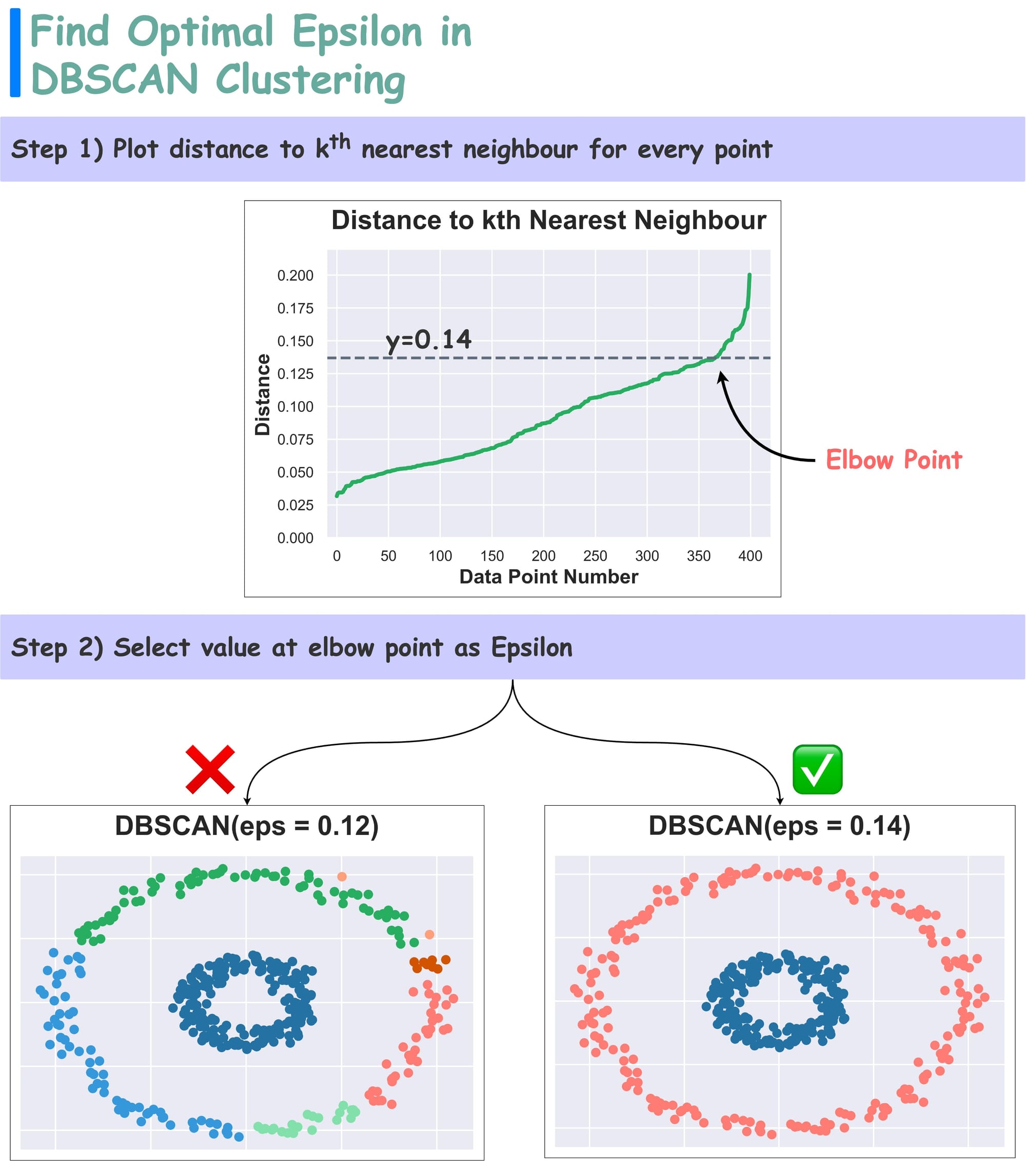
As depicted above, selecting the elbow value provides better clustering results over another value.
Advantages of DBSCAN
- Effective Density-Based Clustering:
- Quite intuitively, DBSCAN excels in separating clusters of high density from those of low density within a given dataset.
- By focusing on the density of data points, it can identify clusters with varying shapes and sizes.
- Robust Outlier Handling:
- DBSCAN is particularly adept at handling outliers within the dataset.
- As discussed earlier, if a data point has no core point close to it, where the core point in itself is an indicator of high density because of the presence of many points in its vicinity, then we can intuitively say that the point will be an outlier.
- In fact, in some cases, DBSCAN is primarily employed as an outlier detection technique. The algorithm's ability to designate noise points as outliers contributes to a more comprehensive understanding of the data's structure.
- We don’t even have to proceed with clustering for outlier detection. Instead, we can just determine if a point is a noise point or not using the parameters
epsilonandminPts.
Disadvantages of DBSCAN
Density-based clustering algorithms have greatly impacted a wide range of areas in data analysis, including outlier detection, computer vision, and medical imaging.
In fact, in many practical applications, as data volumes rise, it can become increasingly difficult to collect labels for supervised learning.
In such cases, non-parametric unsupervised algorithms are becoming increasingly important in understanding large datasets.

However, one of the biggest issues with DBSCAN is its run time.
Until recently, it was believed that DBSCAN had a run-time of $O(n \log n)$ until it was proven to be $O(n^2)$ in the worst case.
Thus, there is an increasing need to establish more efficient versions of DBSCAN.
Although we won’t get into much detail here, it can be proved that DBSCAN can run in $O(n \log n)$ when the dimension is at most $2$, which is rarely the case.
However, it quickly starts to exhibit quadratic behavior in high dimensions and/or when $n$ becomes large.
This can also be verified from the figure below:
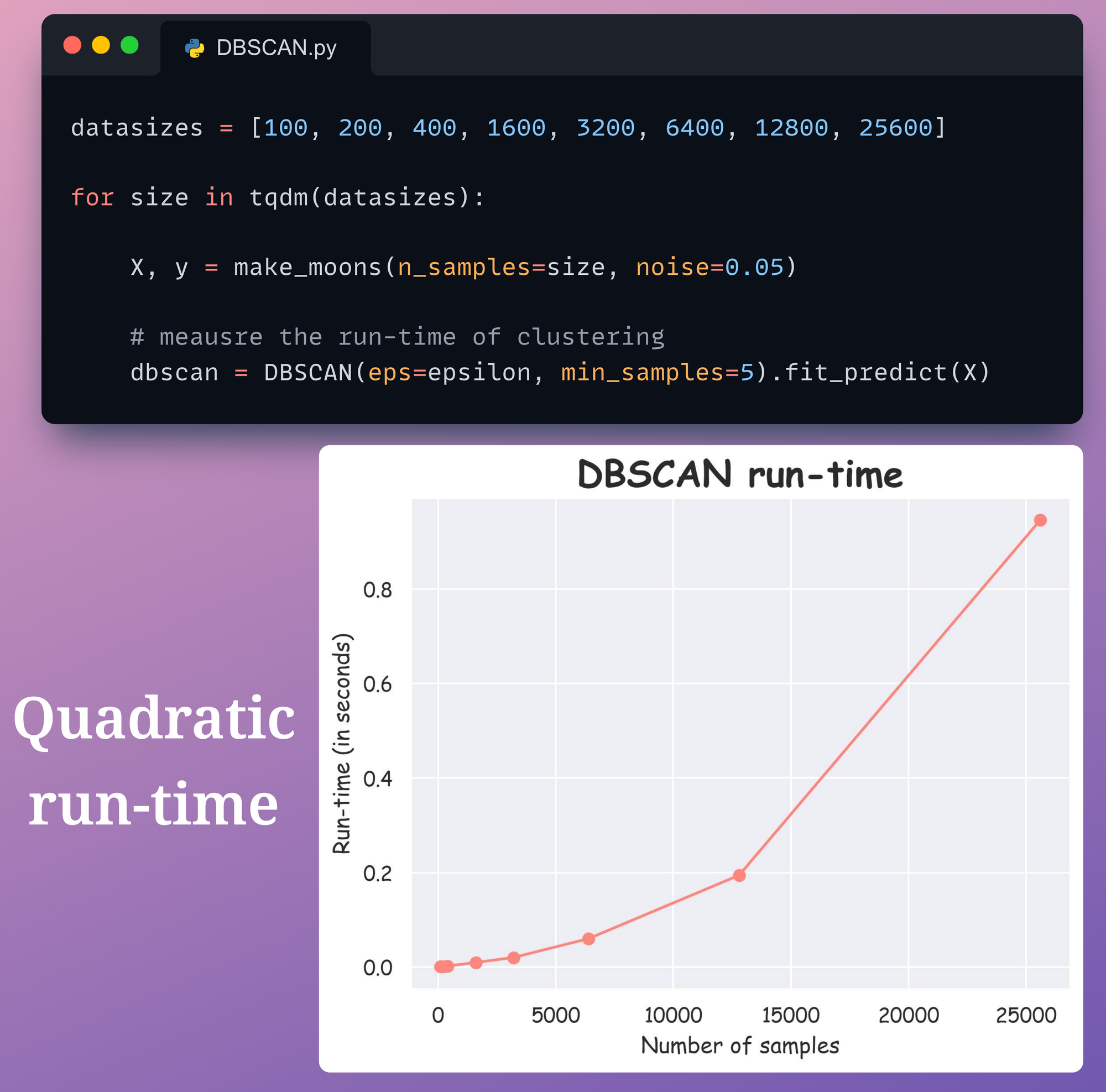
In this experiment, we have a simple 2-dimensional dataset with a varying number of data points.
It is clear that DBSCAN possesses a quadratic run-time with respect to the number of data points.
The quadratic run-time for most density-based algorithms can be realized from the fact that DBSCAN implicitly must compute density estimates for each data point, which is linear time in the worst case for each query.
As discussed above, in the case of DBSCAN, such queries are proximity-based, which are computed for each pair of data points.
This is what gives it a quadratic nature of run-time performance.
DBSCAN++
DBSCAN++ is a step towards a fast and scalable DBSCAN.
Simply put, DBSCAN++ is based on the observation that...

