A Beginner-friendly Introduction to Kolmogorov Arnold Networks (KAN)
What are KANs, how are they trained, and what makes them so powerful?
Introduction
In the last few days, you may likely have at least heard of the Kolmogorov Arnold Networks (KAN). It's okay if you don't know what they are or how they work; this article is precisely intended for that.
However, KANs are gaining a lot of traction because they challenge traditional neural network design and offer an exciting new paradigm to design and train them.
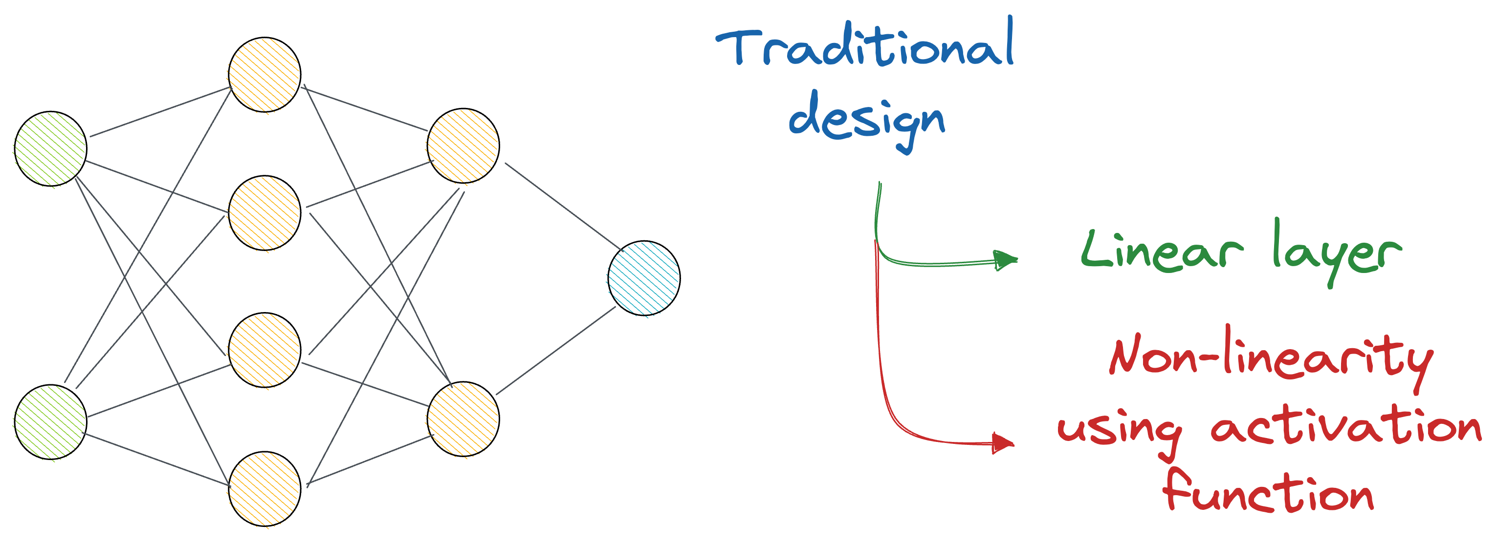
In a gist, the idea is that instead of just stacking many layers on top of each other (which are always linear transformations, and we deliberately introduce non-linearity with activation functions), KANs recommend an alternative approach.
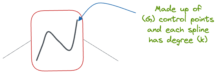
The authors used complex learnable functions (called B-Splines) that help us directly represent non-linear input transformations, with relatively fewer parameters than a traditional neural network.
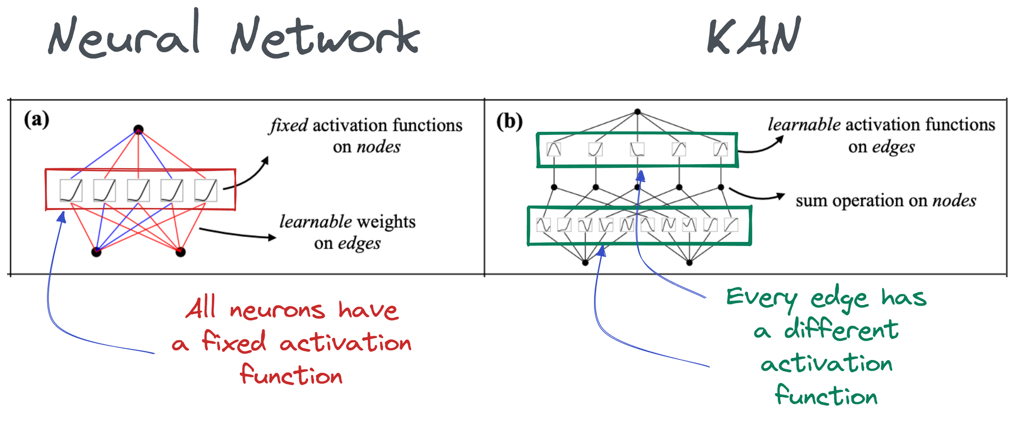
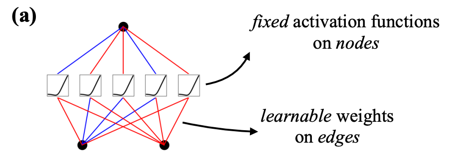
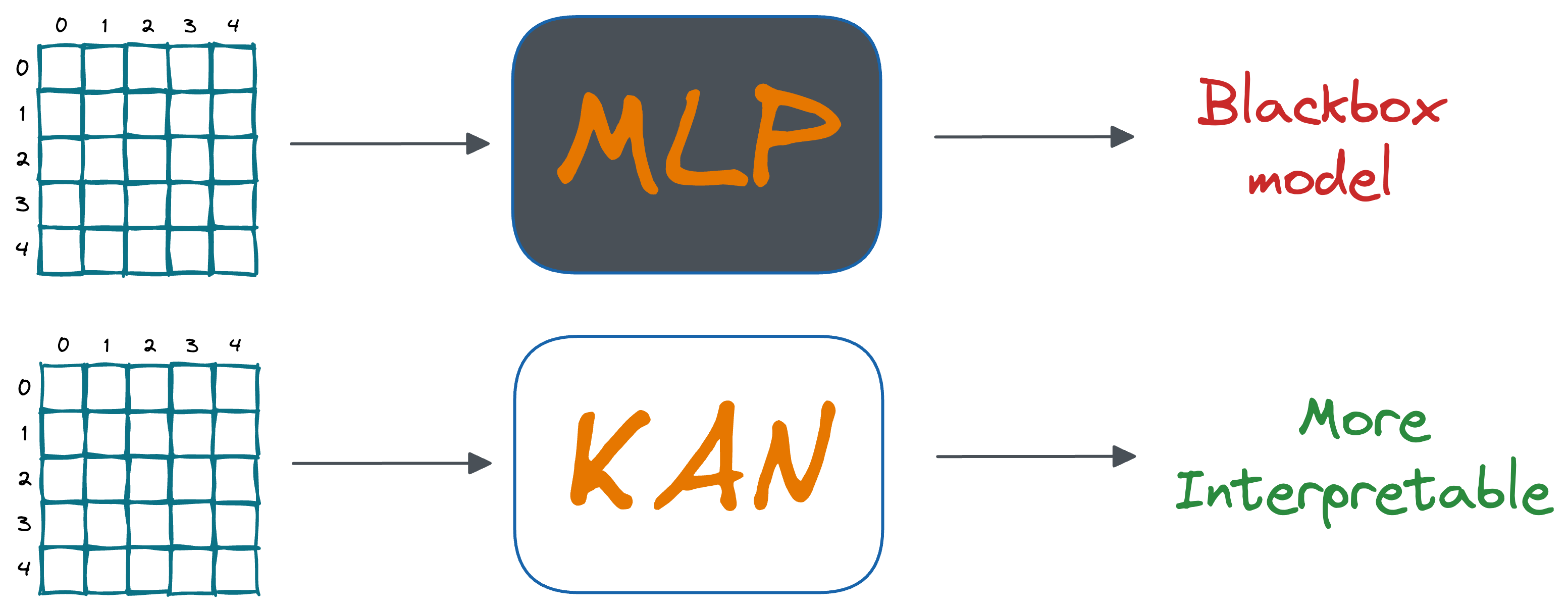
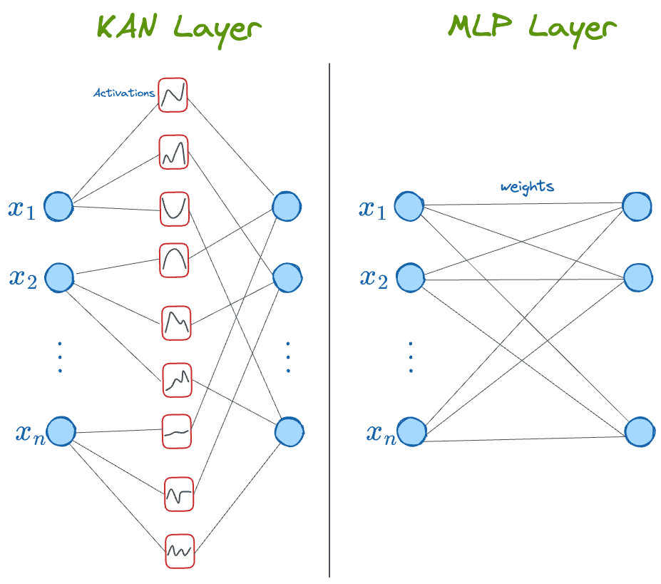
In the above image, if you notice closely:
- In a neural network, activation functions are fixed across the entire network, and they exist on each node (shown below).
- In KAN, however, activation functions exist on edges (which correspond to the weights of a traditional neural network), and every edge has a different activation function.
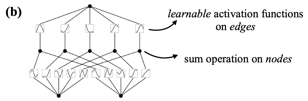
Thus, it must be obvious to expect that KAN is much more accurate and interpretable with fewer parameters.
Going ahead, we shall dive into the technical details of how they work.
Let’s begin!
Universal Approximation Theorem
The universal approximation theorem (UAT) is the theoretical foundation behind the neural networks we use.
In simple words, it states that a neural network with just one hidden layer containing a finite number of neurons can approximate ANY continuous function to a reasonable accuracy on a compact subset of $\mathbb{R}^n$, given suitable activation functions.
The key points are:
- Network Structure: Single hidden layer.
- Function Approximation: Any continuous function can be approximated.
- Activation Function: Must be non-linear and suitable (e.g., sigmoid, ReLU).
Mathematically speaking, for any continuous function $f$ and $\epsilon > 0$, there always exists a neural network $\hat{f}$ such that:
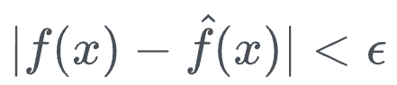
It was only proved for sigmoid activation when it was first proposed in 1989. However, in 1991, it was proven to be applicable to all activation functions.
The fundamental thought process involved here was that a piecewise function can approximate any continuous function on a bounded set.
For instance, the cosine curve between $-\frac{\pi}{2}$ and $\frac{\pi}{2}$ can be approximated with several steps fitted to this curve.
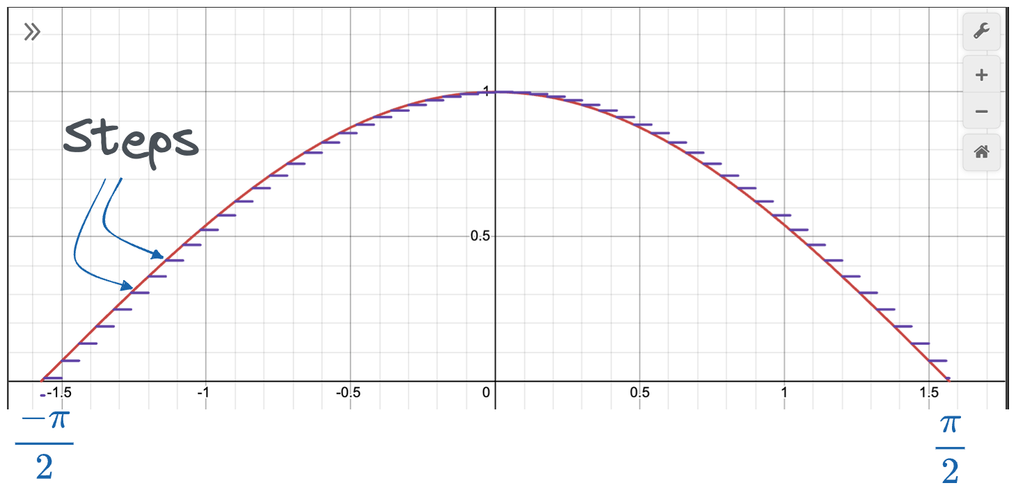
Naturally, the more the number of steps, the better the approximation. To generalize, neural networks with a single hidden layer can map each of its neurons to one piecewise function.
By using weights and biases as gates, each neuron can determine if an input falls within its designated region.
For inputs falling in a neuron’s designated section, a large positive weight will push the neuron’s output towards $1$ when using a sigmoid activation function. Conversely, a large negative weight will push the output towards $0$ if the input does not belong to that section.
While today’s neural networks are much more complex, and large and do not just estimate step functions, there is still some element of “gating” involved, wherein certain neurons activate based on specific input patterns.
Moreover, as more hidden layers are added, the potential for universal approximation grows exponentially — second-layer neurons form patterns based on patterns of first-layer, and so on.
Kolmogorov-Arnold Representation Theorem
This is another theorem that’s based on approximating/representing continuous functions.
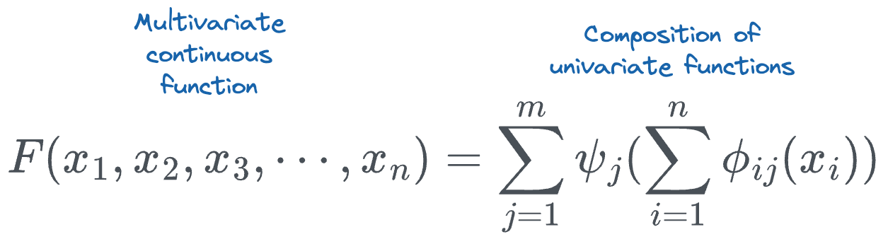
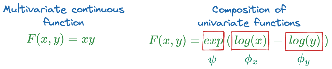
More formally, the Kolmogorov-Arnold representation theorem asserts that any multivariate continuous function can be represented as the composition of a finite number of continuous functions of a single variable.
Let’s break that down a bit:
- "multivariate continuous function" is a function that accepts multiple parameters:
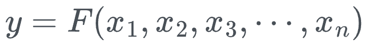
- "a finite number of continuous functions of a single variable" means the following:
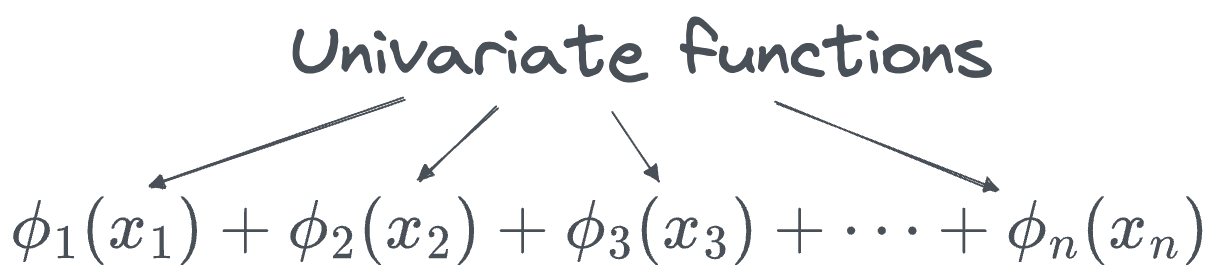
We don't stop here though. The above sum is passed through one more function $psi$:
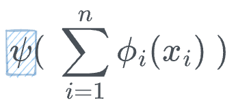
Finally, we also apply a composition to the last step and make this more general as follows:
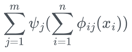
So, to summarize, the Kolmogorov-Arnold representation theorem asserts that any multivariate continuous function can be represented as the composition of continuous functions of a single variable.
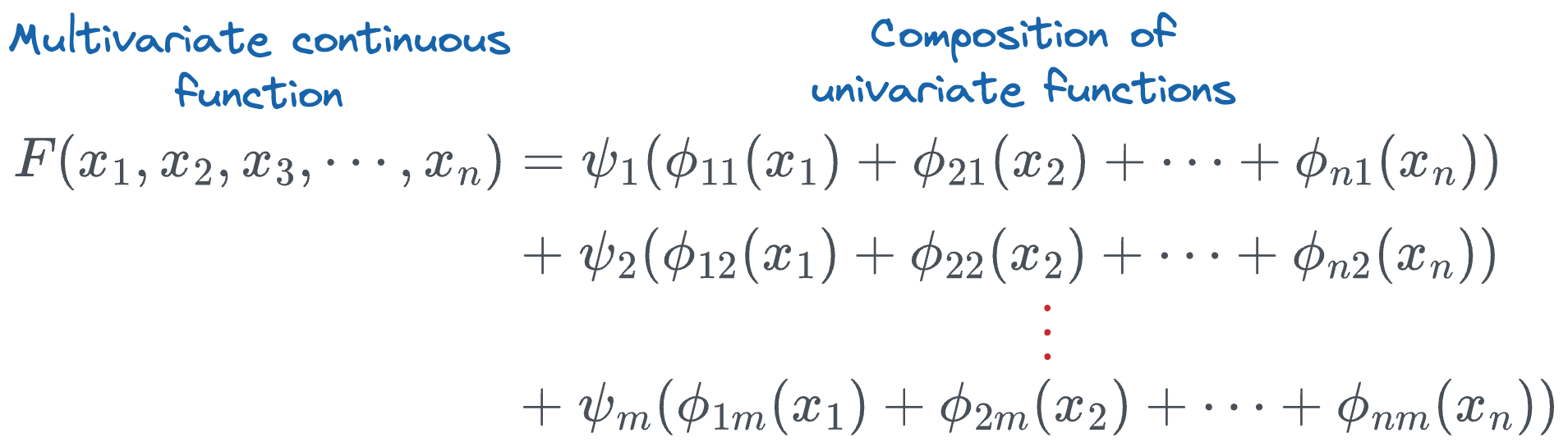
If we expand the sum terms, we get the following:
Here's a simple toy example:
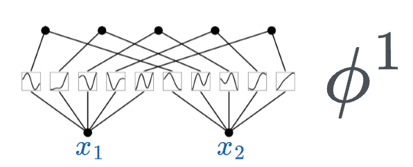
Now, if you go back to the KAN network image shown earlier, this is precisely what's going on in the proposed network.
At first:
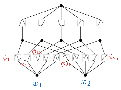
- The input $x_1$ is passed through univariate functions ($\phi_{11}, \phi_{12}, \cdots, \phi_{15}$) to get ($\phi_{11}(x_1), \phi_{12}(x_1), \cdots, \phi_{15}(x_1)$).
- The input $x_2$ is passed through univariate functions ($\phi_{21}, \phi_{22}, \cdots, \phi_{25}$) to get ($\phi_{21}(x_2), \phi_{22}(x_2), \cdots, \phi_{25}(x_2)$).
Next, the two corresponding outputs are aggregated (summed), so the $\psi$ function in this case is just the identity operation ($\psi(z) = z$):
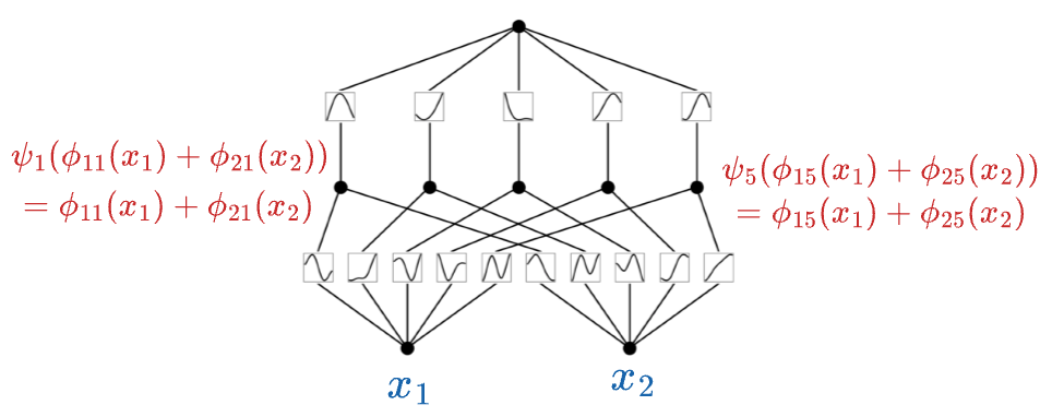
This forms one KAN layer.
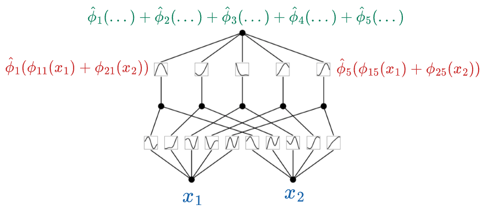
Next, we pass the above output through one more KAN layer.
So the above output is first passed through the $\phi$ function of the next layer and summed to get the final output:
Key Differences
In terms of the scope, the Universal Approximation Theorem applies explicitly to neural networks, while the Kolmogorov-Arnold theorem is a broader mathematical result, which the authors appear to extend to neural networks that supposedly estimate some unknown continuous function.
Talking about the approach, the Universal Approximation Theorem deals with approximating functions using neural networks. In contrast, the Kolmogorov-Arnold theorem provides a way to exactly represent continuous functions through sums of univariate functions, which is expected to make them more accurate.
Finally, from the application perspective, the Universal Approximation Theorem is widely used in machine learning to justify the power of neural networks, while the Kolmogorov-Arnold theorem is aligned towards a theoretical insight that is now being extended to machine learning through architectures like Kolmogorov Arnold Networks.
Thus, since the Kolmogorov-Arnold theorem is more aligned towards exactly representing the multivariate function, embedding it in neural networks is expected to be much more efficient and precise.
In fact, this exact representation could potentially lead to models that can interpreted well and may require fewer resources for training, as the architecture would inherently incorporate the mathematical properties of continuous functions being learned.
How are KANs trained?
Okay, so far, I hope everything is clear.
Quick Summary
Just to reiterate...
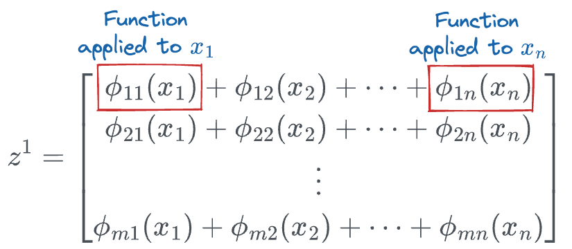
All we are doing in a single KAN layer is taking the input $(x_1, x_2, \cdots, x_n)$ and applying a transformation $\phi$ to it.
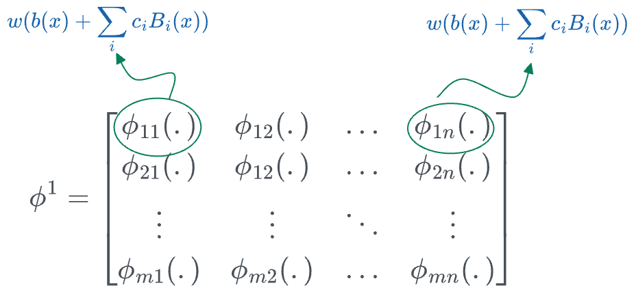
Thus, the transformation matrix $\phi^1$ (corresponding to the first layer) can be represented as follows:
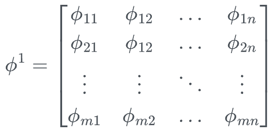
In the above matrix:
- $n$ denotes the number of inputs.
- $m$ denotes the number of output nodes in that layer.
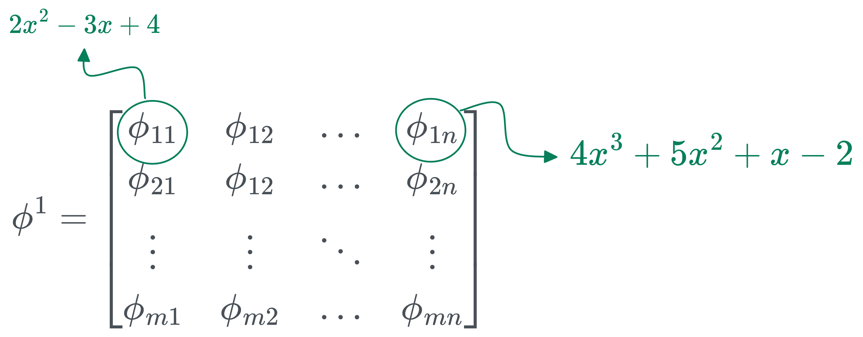
- [IMPORTANT] The individual entries are not numbers, they are univariate functions. For instance:
- $\phi_{11}$ could be $2x^2 - 3x + 4$.
- $\phi_{12}$ could be $4x^3 + 5x^2 + x - 2$.
- and so on...
So to generate a transformation, all we have to do is take the input vector and pass it through the corresponding functions in the above transformation matrix:
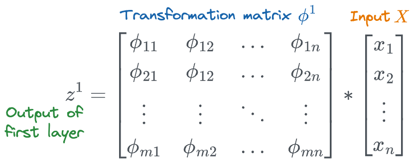
This will result in the following vector:
The above is the output of the first layer, which is then passed through the next layer for another function transformation.
Thus, the entire KAN network can be condensed into one formula as follows:

Where:
- $x$ denotes the input vector
- $\phi^k$ denotes the function transformation matrix of layer $k$.
- $KAN(x)$ is the output of the KAN network.
The above formulation can appear quite similar to what we do in neural networks:

The only difference is that the parameters $\theta^i$ are linear transformations, and $\sigma$ denotes the activation function used for non-linearity, and it is the same activation function across all layers.
In the case of KANs, the matrices $\phi^k$ themselves are non-linear transformation matrices, and each univariate function can be quite different.
But you might be wondering how we train/generate the activation functions that are present on every edge.
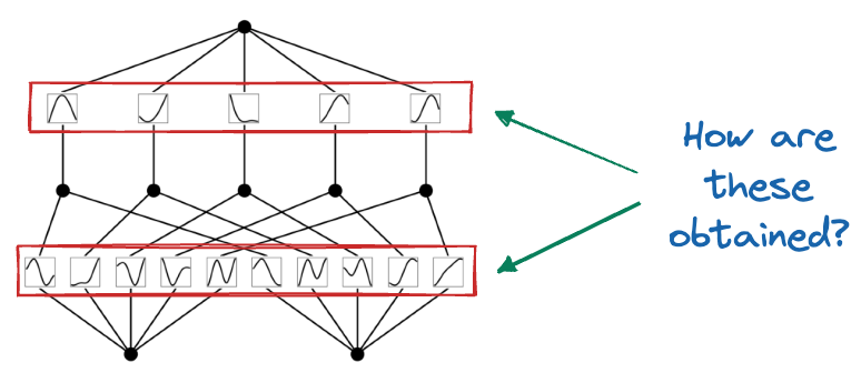
More specifically, how do we estimate the univariate functions in each of the transformation matrices?
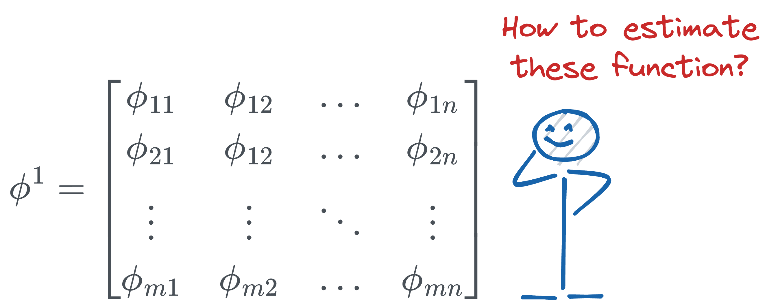
To understand this, we must first understand the concept of Bezier curves and B-Splines.
Bezier curves
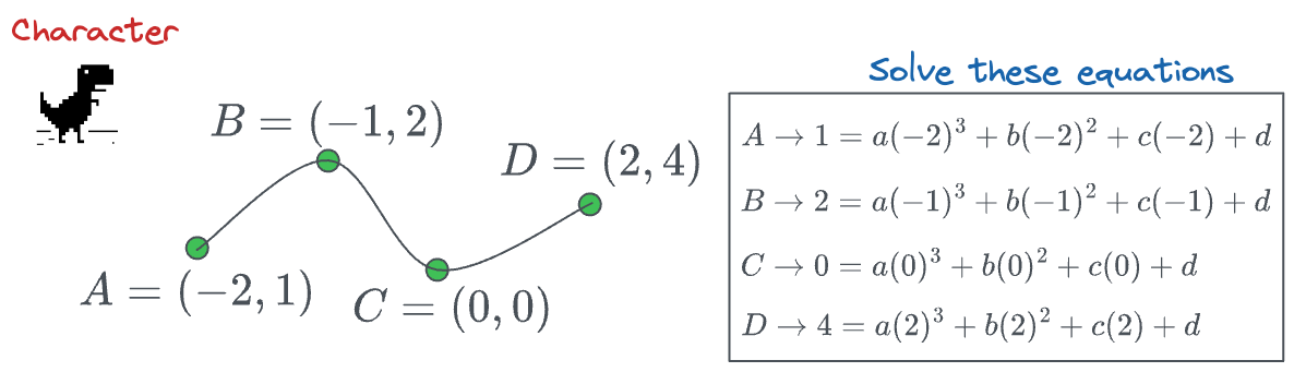
Imagine a gaming character that must pass through the following four points:
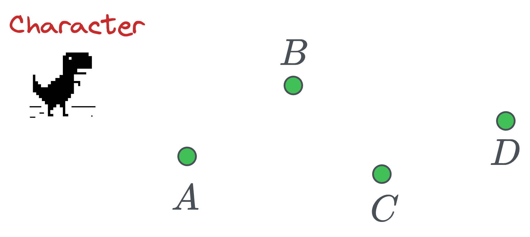
The most obvious way is to traverse them as follows:
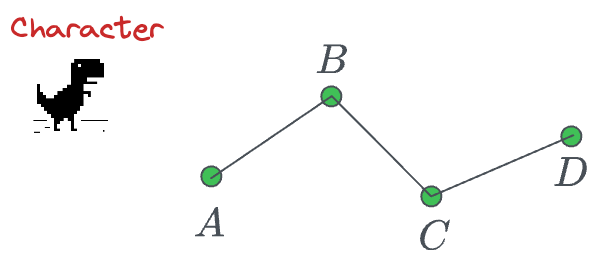
But this movement does not appear natural, does it?
In computer graphics, we would desire a smooth traversal that looks something like this:
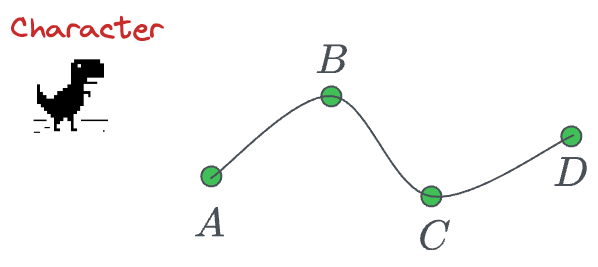
One way to do this is by estimating the coefficients of a higher-degree polynomial by solving a system of linear equations:
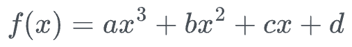
More specifically, we know the location of points $(A, B, C, D)$, so we can substitute them into the above function and determine the values of the coefficients $(a, b, c, d)$.
However, what if we have hundreds of data points?

To formalize a bit, if we have N data points, we must solve $N$ equations to determine the parameters. Solving such a system of linear equations will be computationally expensive and almost infeasible for almost real-time computer graphics applications.
Bezier curves solve this problem efficiently. They provide a way to represent a smooth curve that passes near a set of control points without needing to solve a large system of equations.
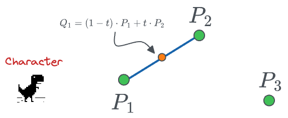
For instance, consider we have these two points, and we need a traversal path:
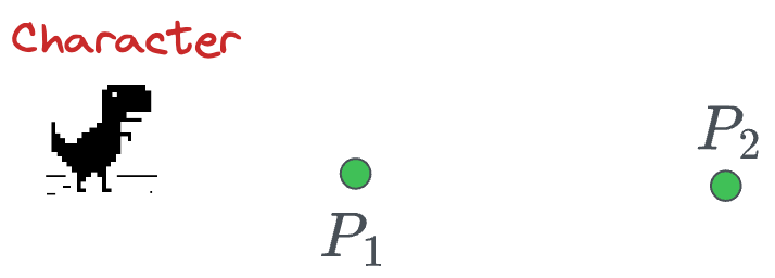
We can determine the curve as follows:
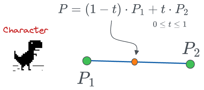
- When $t=0$, the position $P$ will be $P_1$.
- When $t=1$, the position $P$ will be $P_2$.
- We can vary the parameter $t$ from [0,1] and obtain the trajectory.
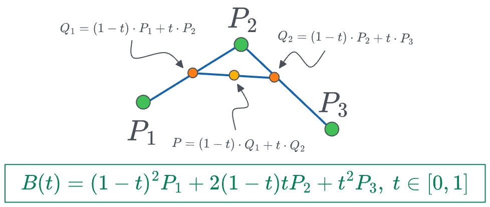
What if we have three points?
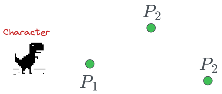
This time, we can extend the above case of 2 points to three points as follows:
- First, we determine a point between $P_1$ and $P_2$ as follows:
- Next, we can determine another point between $P_2$ and $P_3$ as follows:
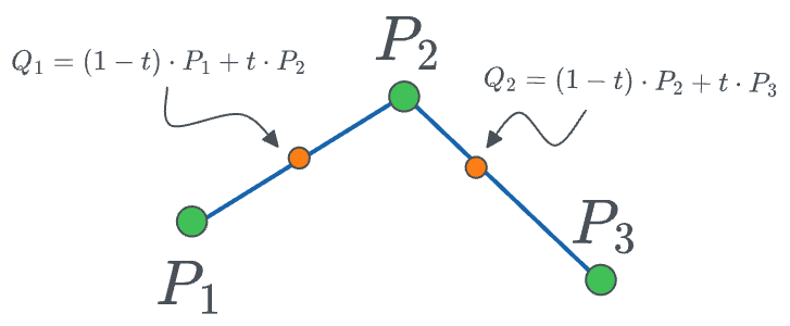
- Finally, between points $Q_1$ and $Q_2$, we can create a linear interpolation:
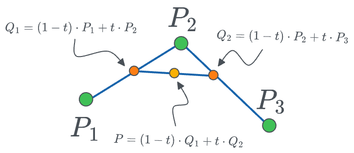
The final curve looks like this:
- We vary $t$ from $[0,1]$ and obtain the red curve.
The final equation for the position of point $P$ is given by:
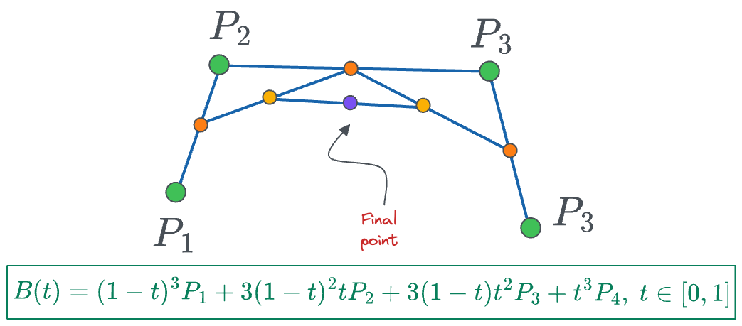
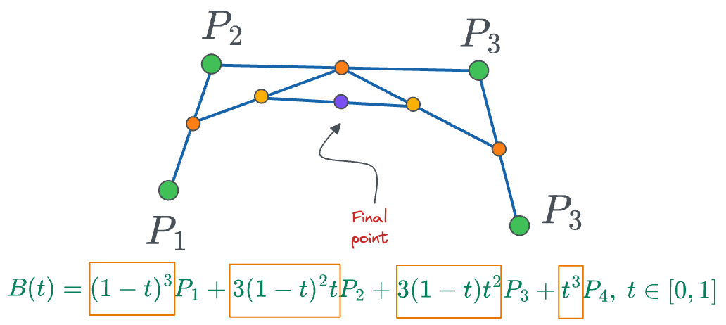
Moving on, the same idea can be extended to 4 points as well to get the following curve:
- We begin by interpolating between
- $P_0$ and $P_1$ to get $Q_1$.
- $P_1$ and $P_2$ to get $Q_2$.
- $P_2$ and $P_3$ to get $Q_3$.
- Next, we interpolate between:
- $Q_1$ and $Q_2$ to get $R_1$.
- $Q_2$ and $Q_3$ to get $R_2$.
- Finally, we interpolate between:
- $R_1$ and $R_2$ to get the final point $P$ (red curve above).
The final formula for the trajectory is given by:
To summarize, these are the trajectory formulas we have obtained so far for 2 points, 3 points, and 4 points:
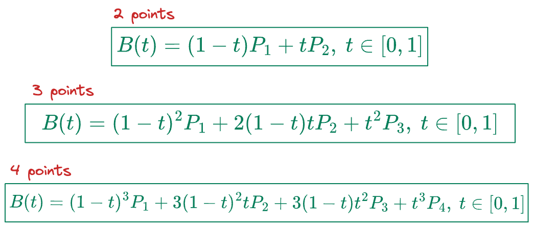
If you notice closely, the coefficients in these formulas match with the binomial coefficients of $(1+x)^n$, so we can extend the above formula for traversal curve to a higher dimension as follows:
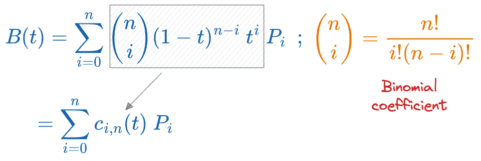
In the above formula, the $c_{i,n}$ is a function of $t$, and at every time stamp, it denotes the contribution of point $P_i$ to the final curve.
Let’s go back to the case where we had 4 points:
If we plot the coefficient terms (marked in yellow boxes above), we get the following plot:
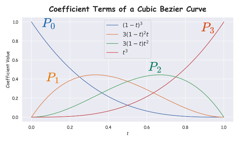
In the above plot, at every timestamp $t$, the plot denotes the contribution of every point to the final curve. For instance:
- At $t=0$, except $P_0$, coefficients of all points are zero, which means the curve starts from $P_0$.
- From $t \in (0.25, 0.5)$, the coefficient of point $P_1$ is max, which means that the curve is closest to $P_1$ in that duration.
- From $t \in (0.5, 0.75)$, the coefficient of point $P_2$ is max, which means that the curve is closest to $P_2$ in that duration.
- At $t=1$, except $P_3$, coefficients of all points are zero, which means the curve ends at $P_3$.
Problem with Bezier curves
Everything looks good so far.
We have a standard formula for bezier curves that can be extended to any number of points:
However, the problem is still the same as before.
Having 100 data points will result in a polynomial of degree 99, which will be computationally expensive. Moreover, the factorial terms are going to be equally hard to compute as well.
We need to find a better way.
B-Splines
B-Splines provide a more efficient way to represent curves, especially when dealing with a large number of data points.
Unlike high-degree polynomials, B-Splines use a series of lower-degree polynomial segments, which are connected smoothly.
In other words, instead of extending Bezier curves to tens of hundreds of data points, which leads to an equally high degree of the polynomial, we use multiple lower-degree polynomials and connect them together to form a smooth curve.
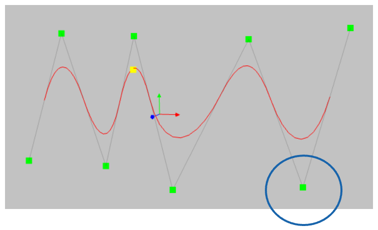
To exemplify, consider the set of data points in the image below:
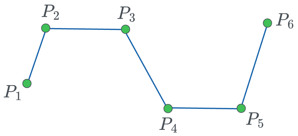
Given that we have 6 points, we can generate a bezier curve of degree 5. That's always an option. However, as discussed above, this is still computationally expensive and not desired.
Instead, we can create curves of smaller degrees (say, 3), and then connect them.
For instance, a full B-spline can be created as follows:
- Some part of it can come from a curve of degree 3 from points $(P_1, P_2, P_3, P_4)$
- Some part of it can come from a curve of degree 3 from points $(P_2, P_3, P_4, P_5)$
- Some part of it can come from a curve of degree 3 from points $(P_3, P_4, P_5, P_6)$
These individual curves are represented below:
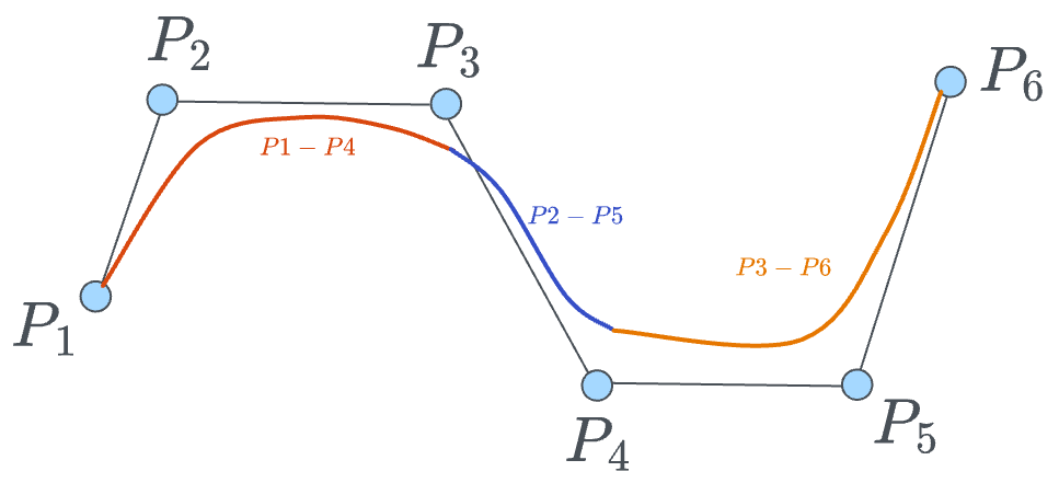
When we have $n$ control pints (6 in the diagram above), and we create $k$ degree polynomial Bezier curves, we get $(n-k)$ Bezier curves in the final Bsplines.
While the actual mathematics behind B-splines is beyond this deep dive, this is a great lecture to understand them in detail:
In a gist, the core idea is to ensure certain continuity conditions at the points where the curves meet.
- Position Continuity ($C^0$ Continuity):
- Ensures that the curves meet at shared points.
- This means ensuring that the end point of the first segment is the same as the starting point of the second segment, and so forth.
- Tangent Continuity ($C^1$ Continuity):
- Ensures that the direction of the curves is consistent at the join points.
- This is achieved by ensuring that the first derivative is continuous at the join points. It is not necessary to ensure this through the curve because the individual Bezier curves are polynomials, so they are always continuous.
- Curvature Continuity ($C^2$ Continuity):
- Ensures that the curvature of the curve is smooth across the joins.
- This involves higher-order derivatives and is more complex but provides even smoother transitions.
Similar to what we saw in Bezier curves, the final B-spline curve is represented as a linear combination of the points $P_i$:
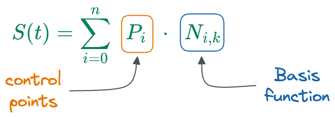
- $P_i$: Control points that define the shape of the curve.
- $𝑁_{𝑖,𝑘}(𝑡)$: B-spline basis functions of degree $k$ associated with each control point $P_i$, and they are similar to what we saw earlier in the case of Bezier curves and are fixed.
Building KAN layer
With those details in mind, we are ready to understand how B-splines are used in KAN to train those higher-degree activation functions.
Recall that whenever we create B-splines, we already have our control points $(P_1, P_2, \dots, P_n)$, and the underlying basis functions based on the degree $k$.
And by varying the position of the control points, we tend to get different curves, as depicted in the video below:
So here's the core idea of KANs:
Let's make the positions of control points learnable in the activation function so that the model is free to learn any arbitrary shape activation function that fits the data best.
That's it.
By adjusting the positions of the control points during training, the KAN model can dynamically shape the activation functions that best fit the data.
- Start with the initial positions for the control points, just like we do with weights.
- During the training process, update the positions of these control points through backpropagation, similar to how weights in a neural network are updated.
- Use an optimization algorithm (e.g., gradient descent) to adjust the control points so that the model can minimize the loss function.
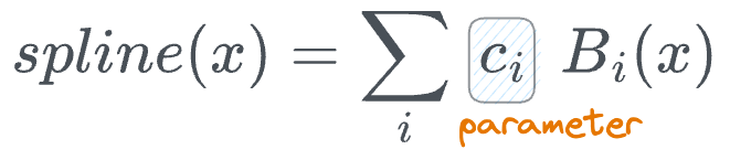
Mathematically speaking, in KANs, every activation function $\phi(x)$ is defined as follows:
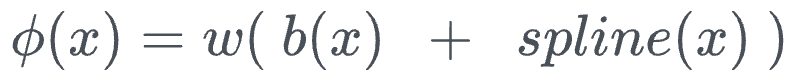
Within this:
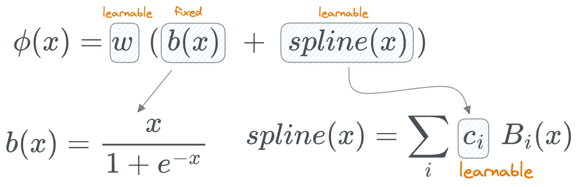
- The computation involves a basis function $b(x)$ (similar to residual connections).
- $spline(x)$ is learnable, specifically the parameters $c_i$, which denotes the position of the control points.
- There's another parameter $w$. The authors say that, in principle, $w$ is redundant since it can be absorbed into $b(x)$ and $spline(x)$. Yet, they still included this $w$ factor to better control the overall magnitude of the activation function.
For initialization purposes:
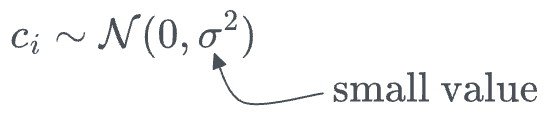
- Each activation function is initialized with $spline(x) \approx 0$. This is done by drawing B-spline coefficients $c_i ∼ \mathcal{N} (0, \sigma^2)$ with a small $σ$ around $0.1$.
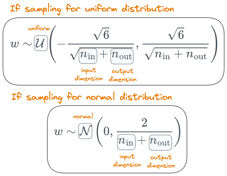
- Moreover, $w$ is initialized according to the Xavier initialization:
Done!
Once this has been defined, the network can be trained just like any other neural network.
More specifically:
- We initialize each of the $phi$ matrices as follows:
- Run the forward pass:

- Calculate the loss and run backpropagation.
Done!
KAN vs MLP
Parameter count
Let's compare the number of parameters of a KAN and MLP, both with $L$ layers and an equal number of neurons in each layer ($N$):
- The number of edges from one layer to another is the same in both cases – $N^2$.
- While the edges of MLP just hold one weight, the edges of KAN hold more parameters because of splines.
- For a B-spline with $G$ control points and degree $k$, the number of basis functions are $G+k-1$. In KAN, as each basis function is associated with one parameter, the number of parameters is also the same – $G+k-1$.
- So, every edge in a KAN holds $G+k-1$ parameters.
- The final parameter count comes out to be as follows (including all layers):
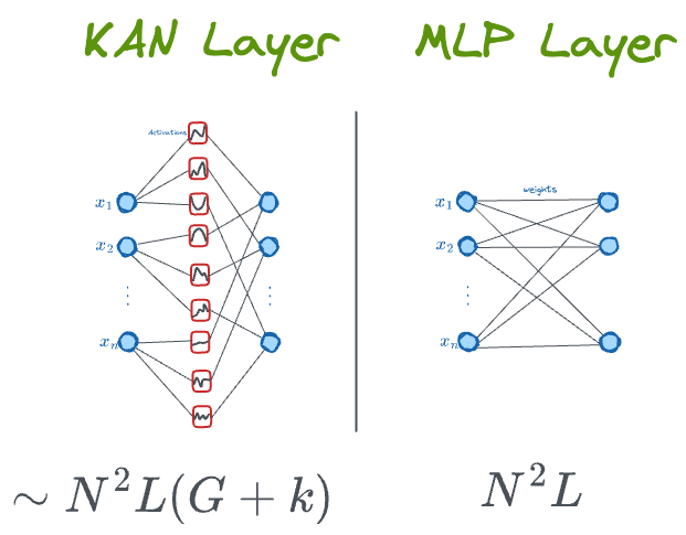
While MLPs appear to be more efficient than KANs, a point to note is that based on their experiments, KANs usually don't require as much large $N$ as MLPs do. This saves parameters while also achieving better generalization.
Performance
The authors have presented many performance-related figures that compare the performance of KANs with MLP on various dummy/toy datasets.
Consider the following image:
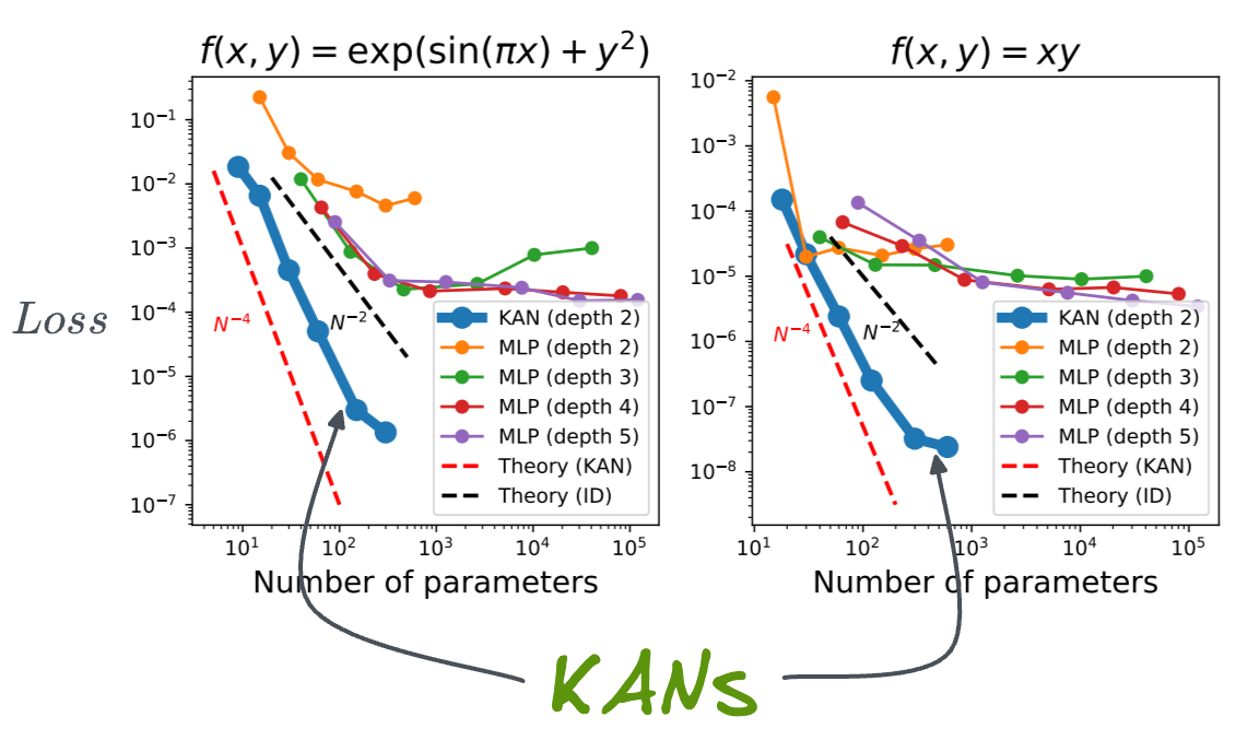
- In both plots,
- KANs consistently outperform MLPs, achieving significantly lower test loss across a range of parameter, and at much lower network depth (number of layers).
- KANs demonstrate superior efficiency, with steeper declines in loss, particularly noticeable with fewer parameters.
- MLP's performance almost stagnates with increasing the number of parameters.
- The theoretical lines, $𝑁^{−4}$ for KAN and $𝑁^{−2}$ for ideal models (ID), show that KANs closely follow their expected theoretical performance.
Here are the results for two more functions:
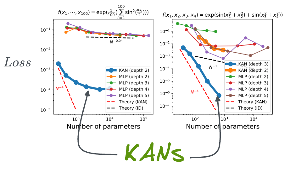
Yet again, in both plots, KANs considerably outperform MLPs by achieving significantly lower test loss across a range of parameter, and at much lower network depth (number of layers).
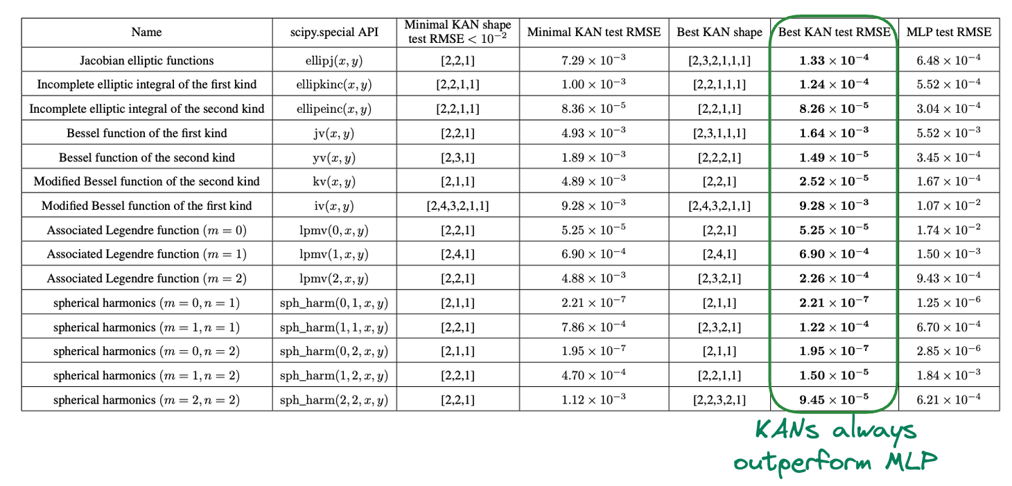
These are some more results across various data shapes, and yet again, KANs' test RMSE is lower than that of MLP.
Continual Learning
Moving on, another incredible thing that KANs possess is continual learning.
For more context, it is commonly observed that when a neural network is trained on a particular task and then shifted to being trained on task 2, the network will soon forget about how to perform task 1.
This happens because there is no notion of locality-storage of knowledge in MLPs, which is found in humans.
Quoting from the paper – “human brains have functionally distinct modules placed locally in space. When a new task is learned, structure re-organization only occurs in local regions responsible for relevant skills, leaving other regions intact. MLPs do not have this notion of locality, which is probably the reason for catastrophic forgetting.”
This is evident from the image below:
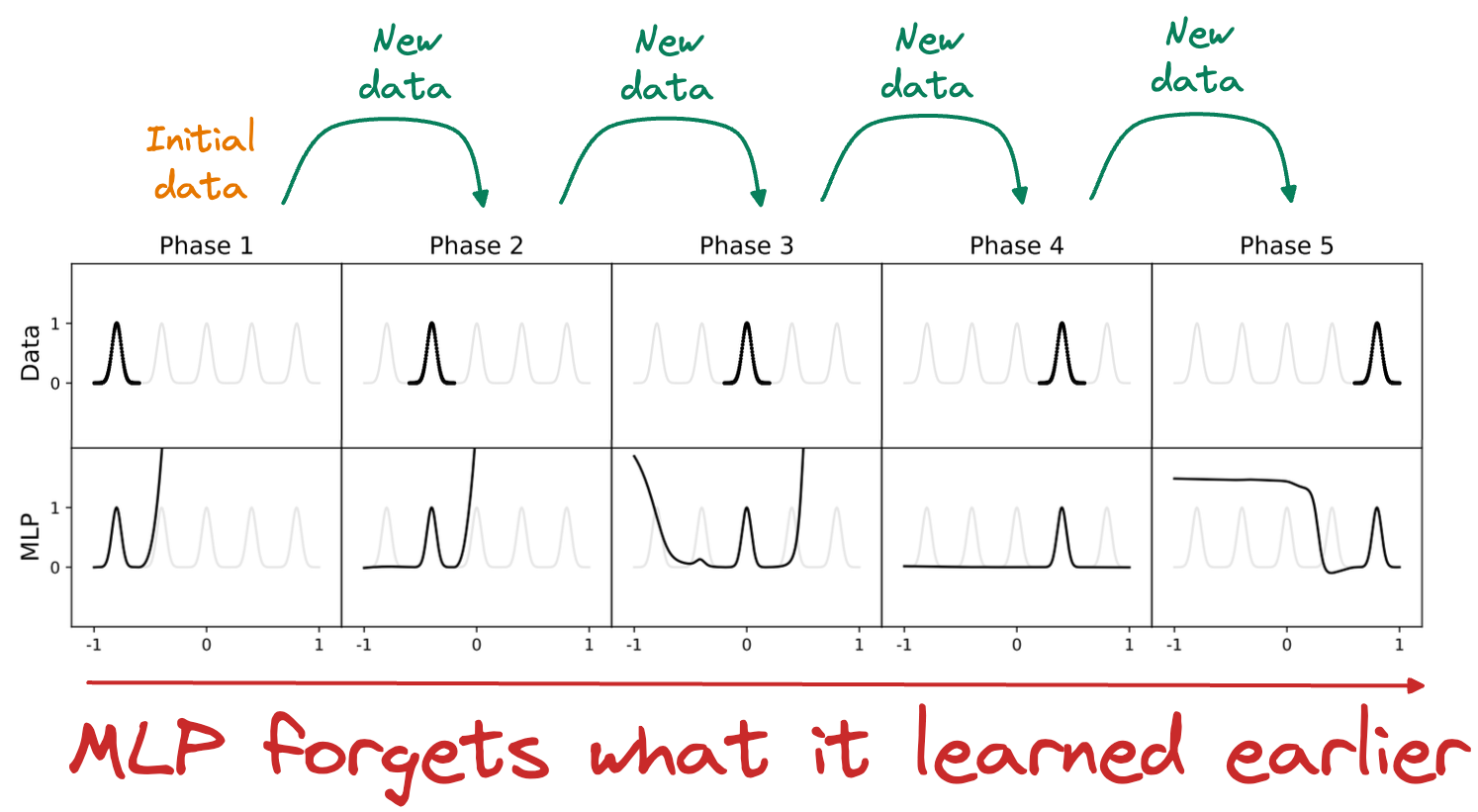
As depicted above, as new data is added, an MLP's learned fit drastically changes.
However, now look at the performance of KANs in the figure below:
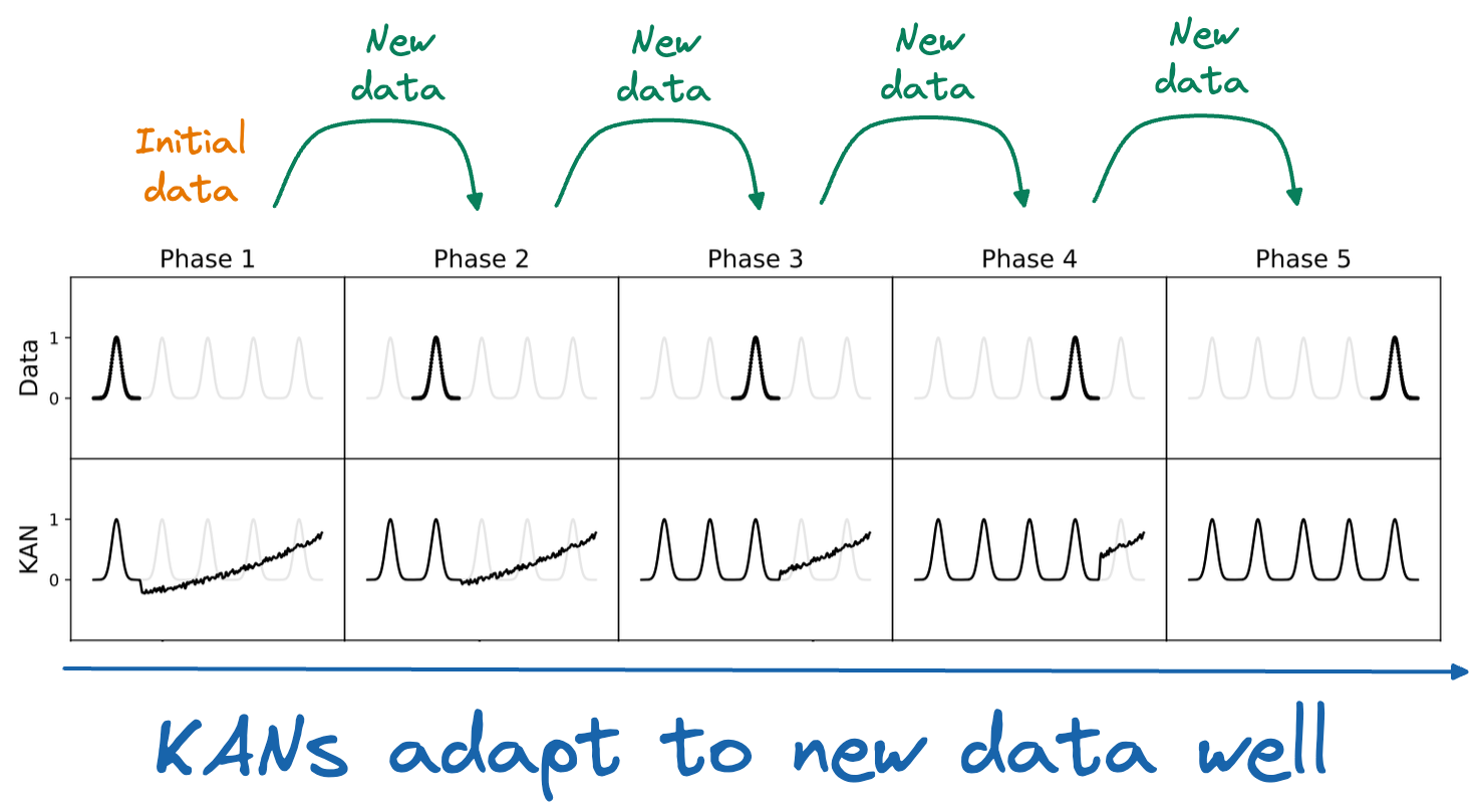
As depicted above, as new data is added, KAN retains the previously learned fit and can also adapt to the new changes.
This happens due to the locality property of B-Splines. To understand better, consider the B-Spline below and notice what happens when I move this point in the animation below this image:
The left part of the B-splines is unaffected by any movement of the above control point.
Since spline bases are local, a sample will only affect a few nearby spline coefficients, leaving far-away coefficients intact (which is desirable since far-away regions may have already stored information that we want to preserve).
However, since MLPs usually use global activations, e.g., ReLU/Tanh/SiLU, etc., any local change may propagate uncontrollably to regions far away, destroying the information being stored there.
This makes intuitive sense as well.
That said, the authors do mention that they are unclear whether this can be generalized to more realistic setups, and they have left investigating this as future work.
Interpretability
Since KANs learn univariate functions at all levels, which can be inspected if needed, it is pretty easy to determine the structure learned by the network using those formulas.
For instance, consider the KAN network below, which learns $f(x, y) = xy$.
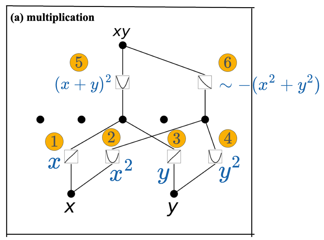
Inspecting the B-splines learned by KAN, we notice the following:
- Both inputs $x$ and $y$ get transformed to their squares in the first KAN later.
- Activation #1 $\rightarrow$ maps $x$ to $x$.
- Activation #2 $\rightarrow$ maps $x$ to $x^2$.
- Activation #3 $\rightarrow$ maps $y$ to $y$.
- Activation #4 $\rightarrow$ maps $y$ to $y^2$.
- In the second layer:
- The sum of Activation #1 and #3, which is $(x+y)$, gets squared by activation #5. This outputs $(x+y)^2$.
- The sum of Activation #2 and #4, which is $(x^2+y^2)$, gets negated by activation #6. This outputs $-(x^2+y^2)$.
- At the output node, we get the final output, which is the sum of activation #5 and activation #6:
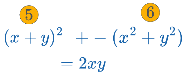
The additional "2" here is just a constant factor and can be adjusted.
For instance, it's possible that activation #5 and #6 learned the following:
- Activation #5 $\rightarrow$ maps input $a$ to $\frac{a^2}{2}$.
- Activation #6 $\rightarrow$ maps input $a$ to $\frac{-a}{2}$.
The scaling factors are not visible to us in the above figure but I hope you get the point.
By inspecting the nodes, we can determine the function learned by the KAN network.
Run-time
The authors of KAN have been honest about one of its biggest bottlenecks, which is its slow training.
They noticed that KANs are usually 10x slower than MLPs when both have the same number of parameters.
However, the overall performance difference could be slight because, as discussed earlier, KANs usually don't require as many parameters as MLPs.
The authors mention that they did not try much to optimize KANs’ efficiency, and they treat bottlenecks more like an engineering problem, which can be improved in future iterations of KAN released by them or the community.
And this did come true.
Within a week's time, someone released an efficient implementation of KAN, called efficient-KAN, which can be found in the GitHub repo below.
 Blealtan
As an exercise, by reading the README of the above repo, can you identify the major bottleneck of the original implementation of KAN, and how this implementation improved it?
Conclusion and Final Thoughts
With this, we come to an end of this deep dive on KANs.
If you have read through so far, you may have understood that KANs are not entirely based on any novel idea but instead based on a common intuition of how neural networks can model data more efficiently, which is quite comprehensible.
While writing this article, I went through a bunch of videos, which I am including here for further reference:
- A quick introduction to KANs:
- For those who understand a bit about KANs, this video distills some of the ongoing discussions since it was released.
- Finally, this is a comprehensive lecture on KANs:
That said, I know we did not discuss much about the code in this article, but I do intend to cover that pretty soon, possibly in an article dedicated to implementing KANs from scratch using PyTorch.
Also, while writing this article, I found this repository, which is a curated list of awesome libraries, projects, tutorials, papers, and other resources related to the Kolmogorov-Arnold Network (KAN).
mintisanAs always, thanks for reading!
Any questions?
Feel free to post them in the comments.
Or
If you wish to connect privately, feel free to initiate a chat here: