Generalized Linear Models (GLMs): The Supercharged Linear Regression

👉

In one of the earlier articles, we formulated the entire linear regression algorithm from scratch.

In that process, we saw the following:

How the assumptions originate from the algorithmic formulation of linear regression.
Why they should not be violated.
What to do if they get violated.
and much more.

Overall, the article highlighted the statistical essence of linear regression and under what assumptions it is theoretically formulated.

Revisiting the linear model and its limitations

Linear regression models a linear relationship between the features $(X)$ and the true/observed output variable $(y)$.

The estimate $\hat y$ is written as:

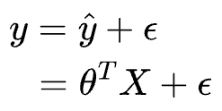
Where:

$y$ is the observed/true dependent variable.
$\hat y$ is the modeled output.
$X$ represents the independent variables (or features).
$θ$ is the estimated coefficient of the model.
$\epsilon$ is the random noise in the output variable. This accounts for the variability in the data that is not explained by the linear relationship.

The primary objective of linear regression is to estimate the values of $\theta=(\theta_1,\theta_2,⋯,\theta_n)$ that most closely estimate the observed dependent variable y.

Talking specifically about the $\epsilon$ – the random noise, we assume it to be drawn from a Gaussian:

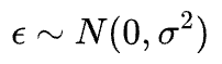
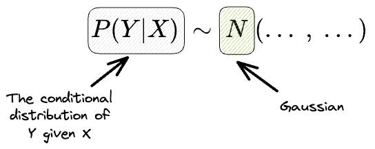
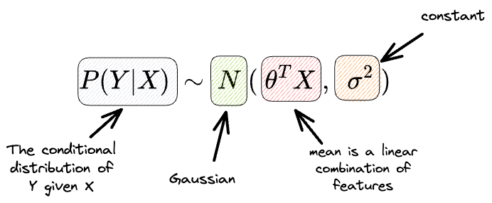
Another way of formulating this is as follows:

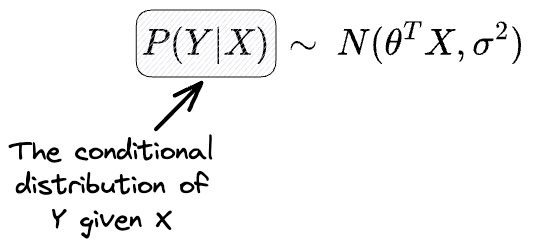
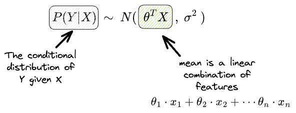
The above says that the conditional distribution of $Y$ given $X$ is a Gaussian with:

Mean = $θ^TX$ (dependent on X).
Variance: $\sigma$ (independent of X or constant).

A graphical way of illustrating this is as follows:

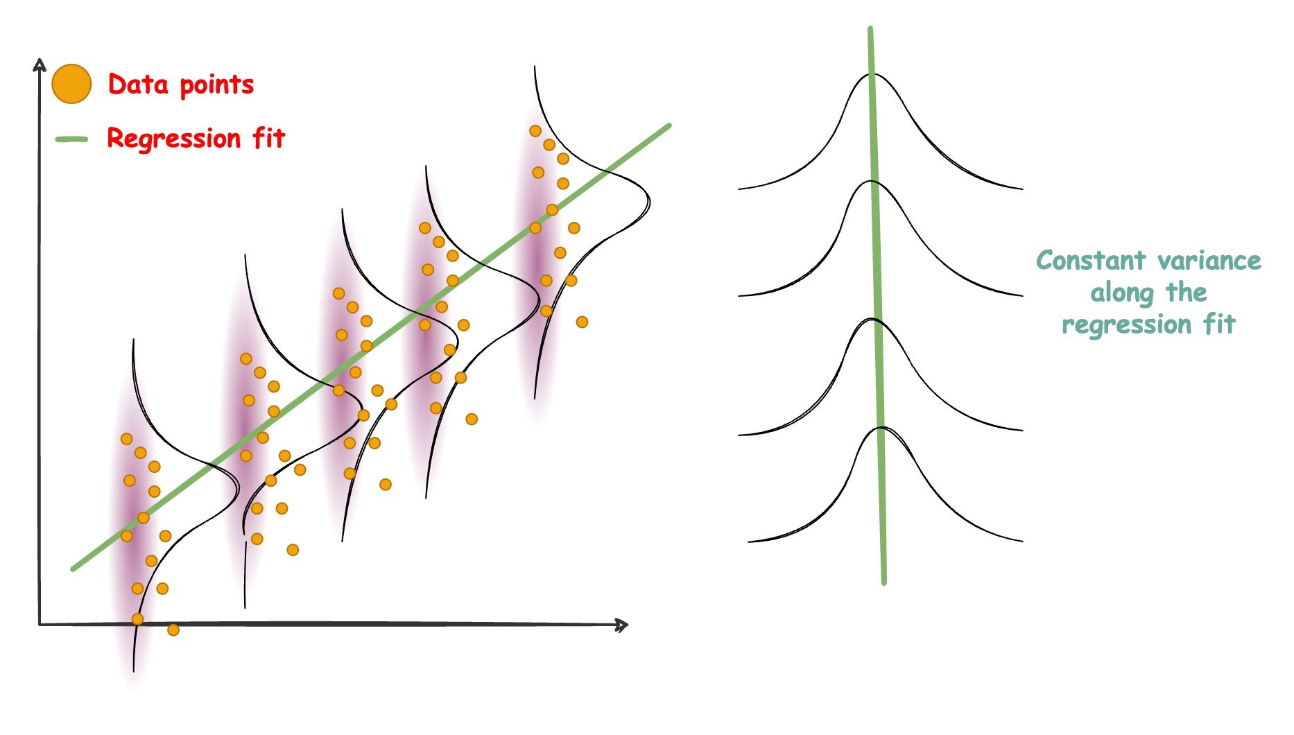
The regression line models the mean of the Gaussian distributions, and the mean varies with $X$. Also, all Gaussians have an equal variance.

So, in a gist, with linear regression, we are trying to explain the dependent variable $Y$ as a function of $X$.

We are given $X$, and we have assumed a distribution for $Y$. $X$ will help us model the mean of the Gaussian.

But it’s obvious to guess that the above formulation raises a limitation on the kind of data we can model with linear regression.

More specifically, problems will arise when, just like the mean, the variance is also a function of $X$.

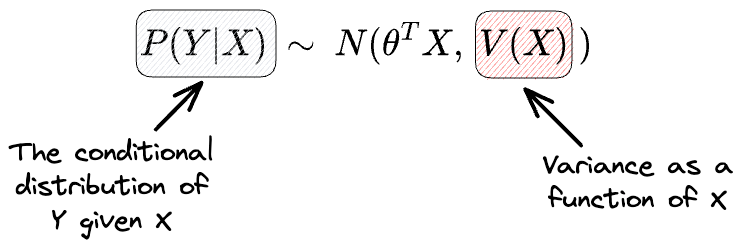
However, during the linear regression formulation, we explicitly assumed that the variance is constant and never depends on $X$.

We aren’t done yet.

There’s another limitation.

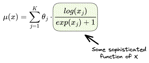
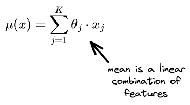
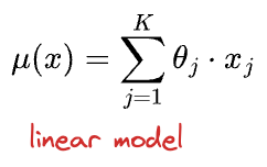
Linear regression assumes a very specific form for the mean. In other words, the mean should be the linear combination of features $X$, as depicted below:

Yet, there’s every chance that the above may not hold true, and instead, the mean is represented as follows:

So, to summarize, we have made three core assumptions here:

#1) If we consider the conditional distribution $P(Y|X)$, we assume it to be a Gaussian.

#2) $X$ affects only the mean, that too in a very specific way, which is linear in the individual features $x_j$.

#3) Lastly, the variance is constant for the conditional distribution $P(Y|X)$ across all levels of $X$.

But nothing stops real-world datasets from violating these assumptions.

In many scenarios, the data might exhibit complex and nonlinear relationships, heteroscedasticity (varying variance), or even follow entirely different distributions altogether.

Thus, we need an approach that allows us to adapt our modeling techniques to accommodate these real-world complexities.

Generalized linear models attempt to relax these things.

More specifically, they consider the following:

What if the distribution isn’t normal but some other distribution from the exponential family?
What if $X$ has a more sophisticated relationship with the mean?
What if the variance varies with $X$?

Let’s dive in!

Generalized linear models

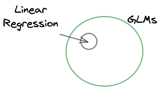
As the name suggests, generalized linear models (GLMs) are a generalization of linear regression models.

Thus, the linear regression model is a specific case of GLMs.

They expand upon the idea of linear regression by accommodating a broader range of data distributions.

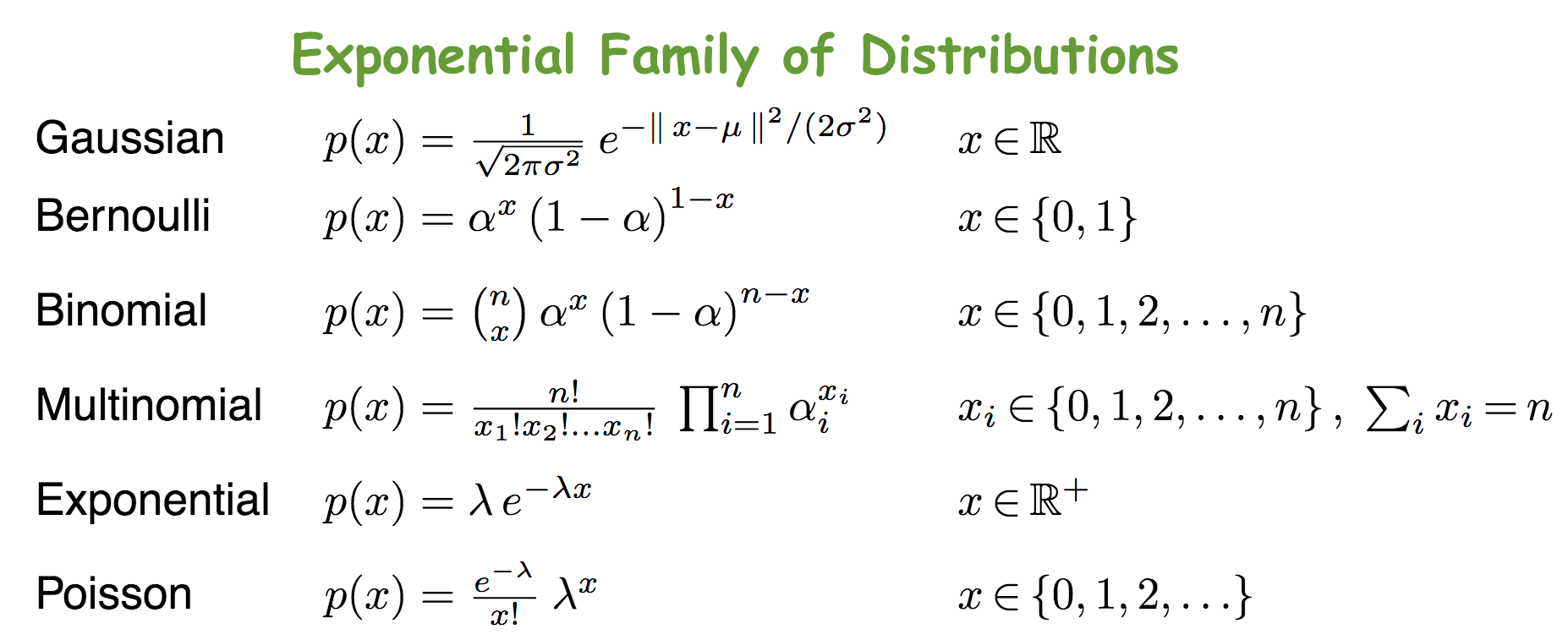
Unlike traditional linear regression, which assumes that the response variable follows a normal distribution and has a linear relationship with the predictors (as discussed above), GLMs can handle various response distributions – Binomial, Poisson, Gamma distributions, and more.

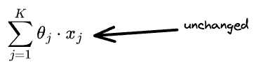
However, before proceeding ahead, it is essential to note that with GLMs, the core idea remains around building “linear models.” Thus, in GLMs, we never relax the linear formulation:

We don't change the linear formulation in GLMs

We’ll understand why we do this shortly.

So what do we change?

In GLMs, the first thing we relax is the conditional distribution $P(Y|X)$, which we assumed to be a Gaussian earlier.

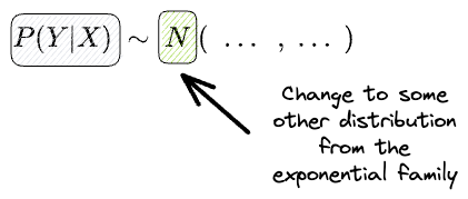
We change the normal distribution to some other distribution from the exponential family of distributions, such as:

Some members of the exponential family of distributions

Why specifically the exponential family?

Because as we would see ahead, everything we typically do with the linear model with Gaussian extends naturally to this family. This includes:

The way we formulate the likelihood function
The way we derive the maximum likelihood estimators, etc.

But the above formulation gets extremely convoluted when we go beyond these distributions.

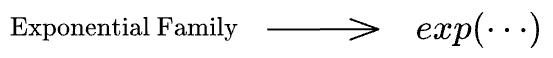
This is because, as the name suggests, the probability density functions (PDFs) of distributions in the exponential family can be manipulated into an exponential representation.

This inherent structure simplifies the mathematical manipulations we typically do in maximum likelihood estimation (MLE):

#1) Define the likelihood function for the entire dataset: Here, we typically assume that the observations are independent. Thus, the likelihood function for the entire dataset is the product of the individual likelihoods.
#2) Take the logarithm (the obtained function is called log-likelihood): To simplify calculations and avoid numerical issues, it is common to take the logarithm of the likelihood function. This step gets simplified if the likelihood values have an exponential term — which the exponential family of distributions can be manipulated to possess.

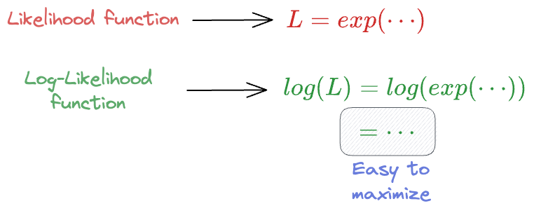
If the likelihood function has exponents, it is easy to maximize the log-likelihood

#3) Maximize the log-likelihood: Finally, the goal is to find the set of parameters $\theta$ that maximize the log-likelihood function.

More specifically, when we take the logarithm in the MLE process, it becomes easier to transform the product in the likelihood function into a summation. This can be further simplified with the likelihood involving exponential terms.

We also saw this in one of the earlier articles:

Lastly, the exponential family of distributions can explain many natural processes.

This family encapsulates many common data distributions encountered in real-world scenarios.

Count data $\rightarrow$ Poisson distribution may help.
Binary Outcomes $\rightarrow$ Bernoulli distribution.
Continuous Positive-Valued Data $\rightarrow$ Gamma distribution.
The time between events $\rightarrow$ try Exponential Distribution.

So overall, we alter the specification of the normal distribution to some other distribution from the exponential family.

There's another thing we change.

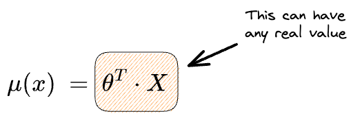
Earlier, we had the formulation that the mean is directly the linear combination of the features.

In GLMs, we extend it to the idea that some function of the mean is the linear combination of the features.

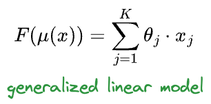
Here, $F$ is called the link function.

While the above notation of putting the link function onto the mean may not appear intuitive, it’s important to recognize that this approach serves a larger purpose within GLMs.

By putting the transformation on mean instead, we maintain the essence of a linear model intact while also accommodating diverse response distributions.

Understanding the purpose of the link function is also simple.

Imagine you had the Bernoulli random variable for the condition distribution of $Y$ given $X$.

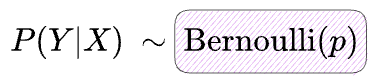
We know that its mean ($p$ or $\mu(x)$) will always lie between [0,1].

However, if we did not add a link function and instead preferred the following representation, the mean can have any real value as $\theta^T \cdot X$ can span all real values.

What the link function does is it maps the mean ($\mu(x)$), which is constrained to some specific range, to all possible real values so that the compatibility between the linear model and the distribution’s mean is never broken.

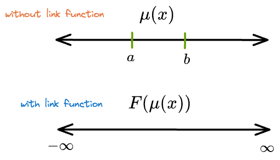
Map the mean to all real values using the link function

That is why they are also called “link” functions. It is because they link the linear predictor $\theta^T \cdot X$ and the parameter for the probability distribution $\mu(x)$.

Thus, to summarize, there are three components in GLMs.