If you consider the last decade (or 12-13 years) in machine learning, neural networks have quite clearly dominated the narrative in many discussions, often being seen as the go-to approach for a wide range of problems.
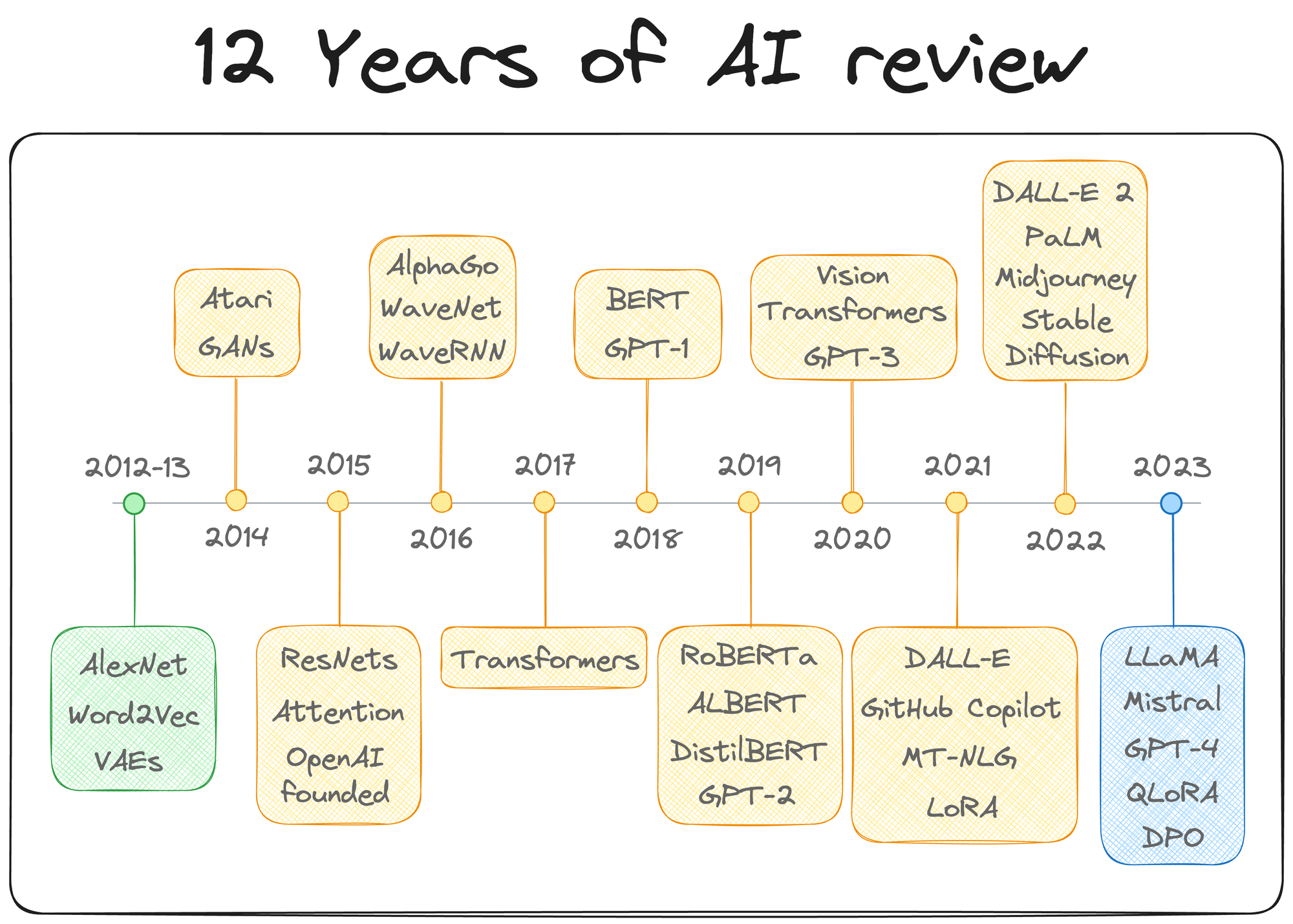
This is a timeline I recently published highlighting some of the major events in the last 12 years, and you would hardly find any major event that did not involve neural networks:
In contrast, tree-based methods tend to be perceived as more straightforward, and as a result, they don't always receive the same level of admiration.
However, in practice, tree-based methods frequently outperform neural networks, particularly in structured data tasks.
This is a well-known fact among Kaggle competitors, where XGBoost, a powerful implementation of gradient boosting, has become the tool of choice for top-performing submissions.
One would spend a fraction of the time they would otherwise spend on models like linear/logistic regression, SVMs, etc., to achieve the same performance as XGBoost.
Given how dominant this one algorithm has been in tabular, I feel it is quite important to know how it was put together and what makes it so powerful.
This is a complete deep dive on XGBoost, wherein:
- We will formulate the entire XGBoost algorithm from scratch.
- Moreover, to solidify that understanding, we shall implement the XGBoost algorithm without native implementations.
Background
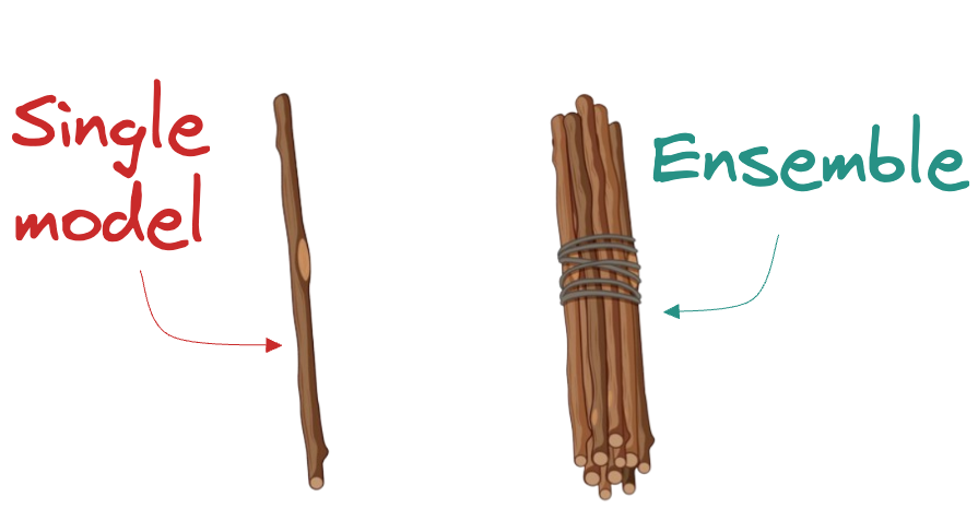
Whenever I want to intuitively illustrate the power of ensemble models to someone, I show this image.
Tree-based ensembles, or rather, I should say, boosting algorithms, have been one of the most significant contributions to tabular machine learning.
The reason why I did not include bagging algorithms is because in my personal experience, I have rarely found them to be on par in comparison to boosting algorithms.
And it isn't hard to understand the reason behind this.
Let's dive in!
Why Boosting > Bagging?
Consider the diagram below, which illustrates the idea of bagging:
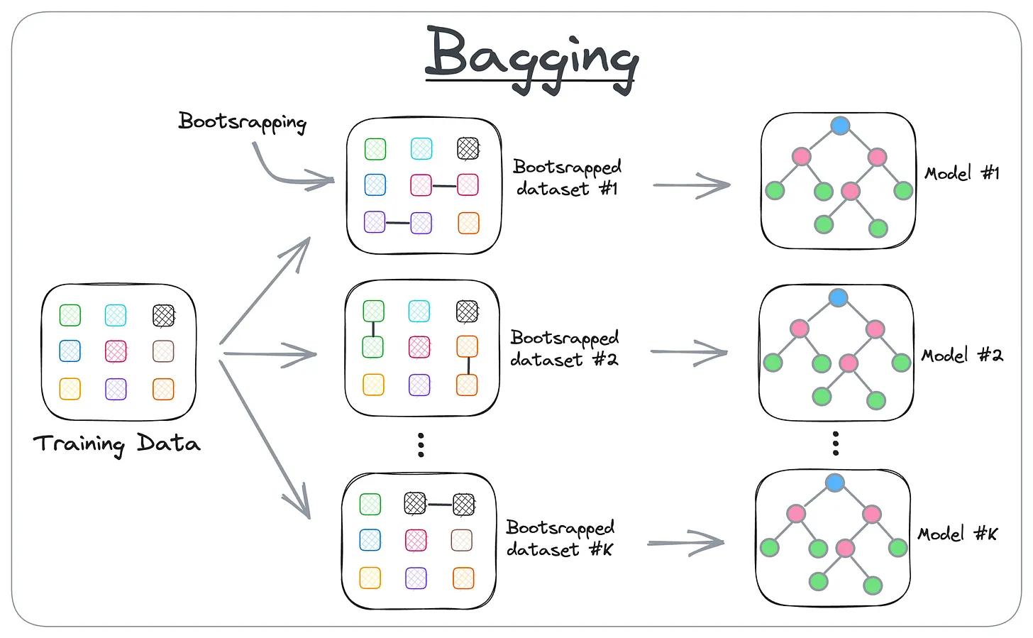
- Step 1: create different subsets of data (this is called bootstrapping).
- Step 2: Train one model per subset.
- Step 3: Aggregate all predictions to get the final prediction.
Training every tree independently makes the overall training procedure of a random forest (or ExtRa Trees, which is slightly different from a random forest) a highly parallelizable operation.
However, this is precisely where the biggest bottleneck with Bagging lies.
More specifically, since every tree is independently trained on a random subset of the data, the diversity among the trees tends to be higher (which is what leads to a model with low variance), but one tree in the ensemble has no idea about what the other tree is struggling with or good at:
If one tree is already good at something, it is better to focus on other parts of the dataset that have not been fully captured yet.
This leads to a suboptimal performance, or even if the performance is satisfactory, we end up creating many more trees than what is needed.
We also discussed this in the daily newsletter:
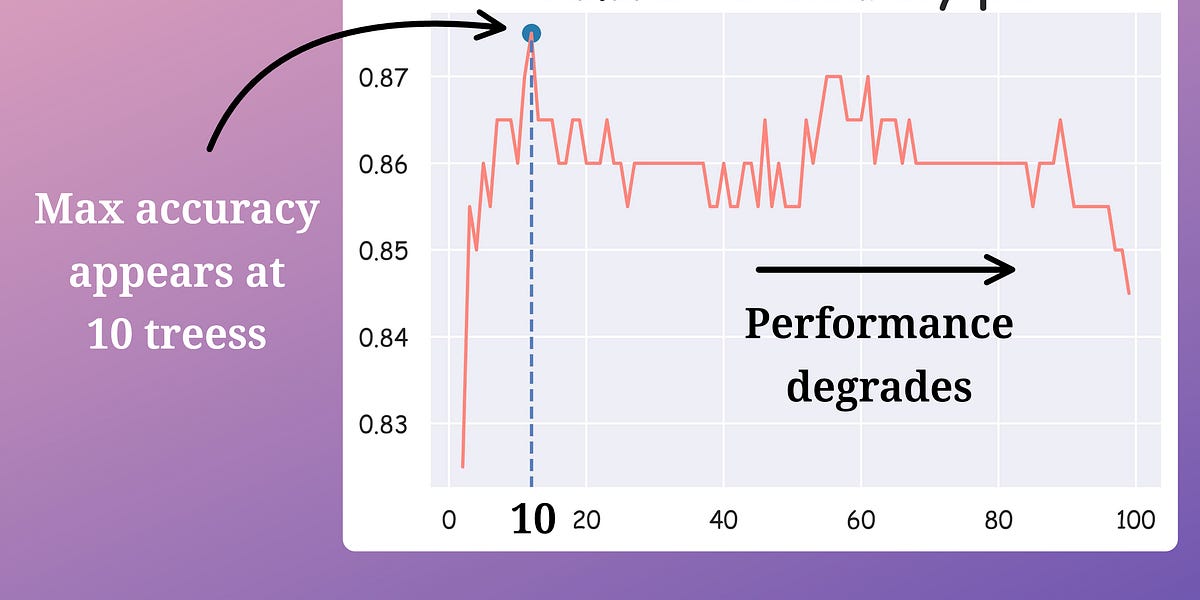
To recall, we removed trees from a random forest model while increasing the accuracy and reducing the prediction time:
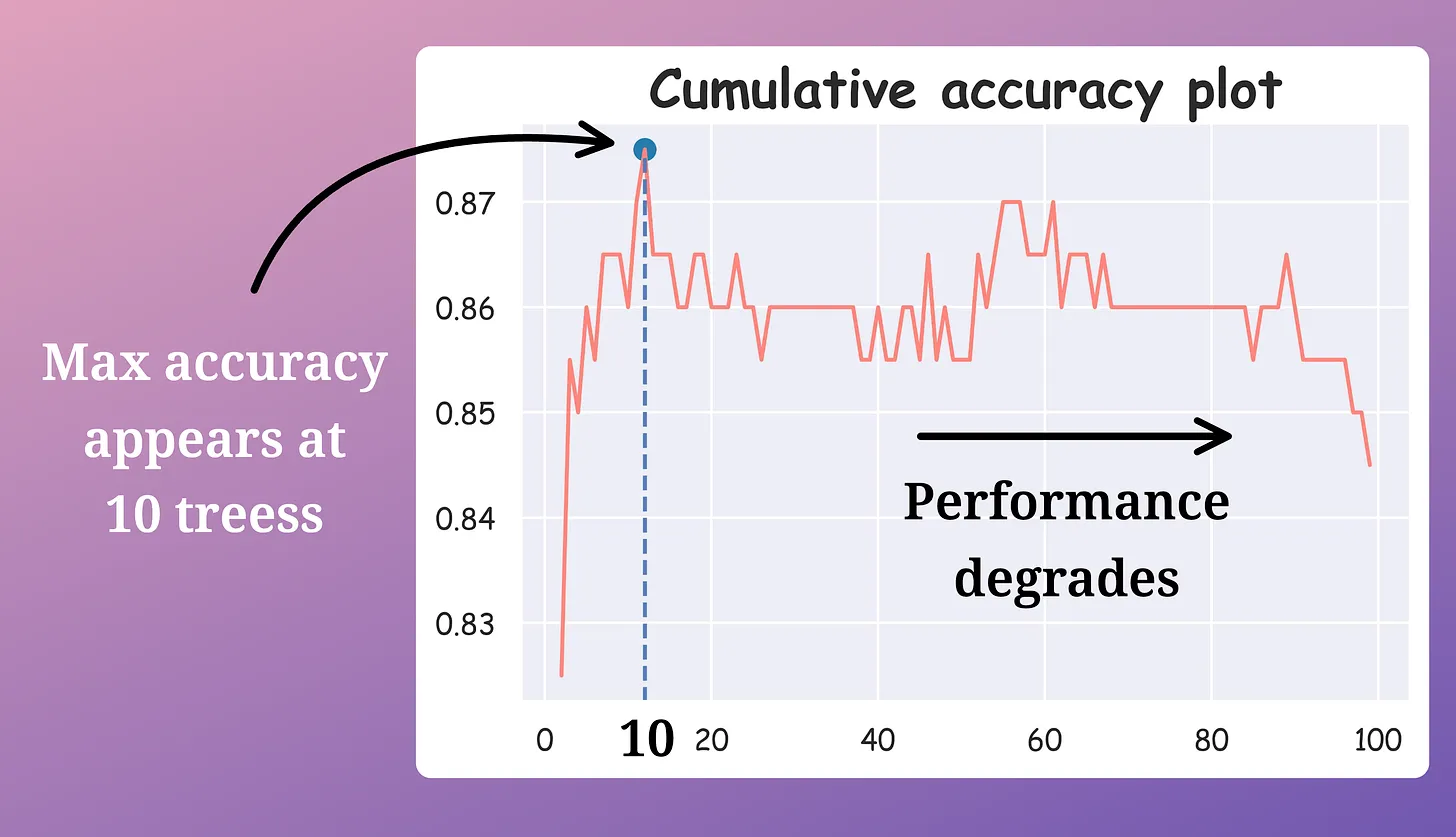
Here's how we did this:
- We calculate the validation accuracy of every decision tree in the random forest model.
- We arranged the accuracies in decreasing order.
- We kept only the “k” top-performing decision trees and removed the rest (while considering another out-of-bag performance to avoid overfitting the validation test).
After doing this, we were left with the best-performing decision trees in our random forest.
We can also understand why bagging leads to suboptimal performance with a real-life analogy.
Consider an ensemble as a group of students who are supposed to appear for an exam together (a group exam).
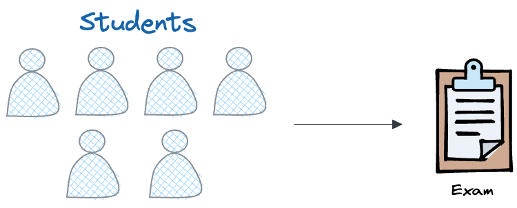
Which of the following is a wiser thing to do:
- Approach 1: Each student will study a subset of the syllabus independently.
- Approach 2: Students communicate and collaborate. One's weaknesses are covered by another student.
It isn't difficult to tell which one is better:
- While approach 1 ensures coverage of the entire syllabus, the students will overlap in what they study, leading to redundant efforts and gaps in knowledge. This is akin to how bagging works—each tree (or student) operates independently, potentially missing out on the opportunity to build on the strengths of others.
- However, with approach 2, after the first student takes a practice test and identifies weak areas, the next student focuses on those gaps, and so on. By the time the last student prepares, the group as a whole has a much stronger grasp of the entire syllabus.
This collaborative approach is the essence of boosting algorithms, which is depicted in the diagram below:
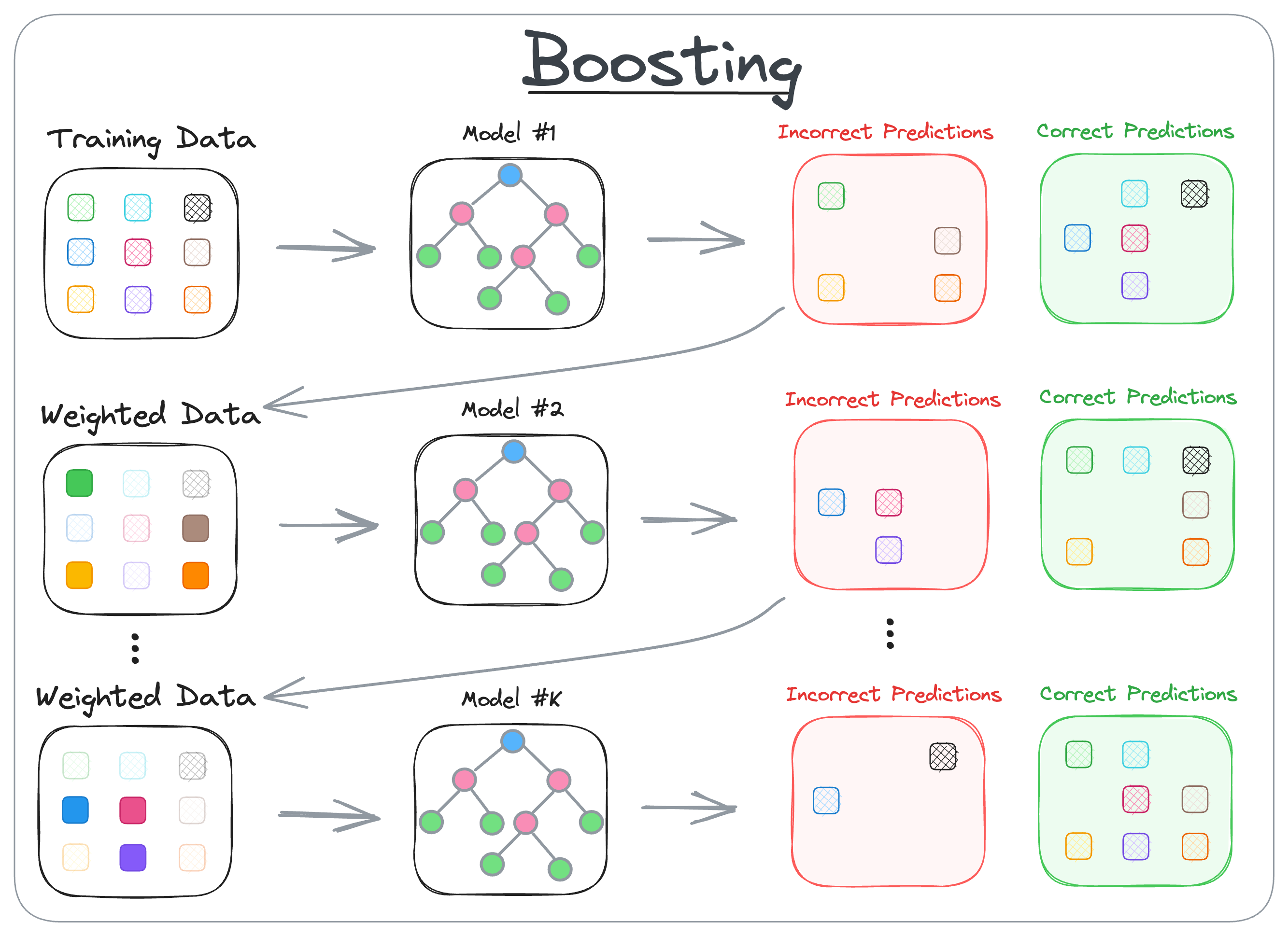
As depicted above, boosting builds trees sequentially, where each tree is trained to correct the errors made by the previous ones.
In fact, this technique is found to be so powerful that they are often observed to be on par with neural networks in terms of performance and generalization.
While they are many variants of boosting, like:
- AdaBoost, which we have already discussed in the newsletter here: A Visual Guide to AdaBoost.
- LightGBM
- CatBoost...
...the focus of this deep dive is XGBoost, which is my go-to boosting algorithm almost always.
There are only a few variable factors in a tree-based boosting model:
- How you construct each tree: This includes decisions about which features to split on at each level and the splitting criteria.
- How to construct the next tree based on the current trees: The variable here is the loss function, which guides the model on how to focus the next tree to correct the errors of the previous ones.
- How to weigh the contribution of each tree in the final model: This determines the influence of each tree in the overall ensemble.
That’s mostly it!
Vary the design choices for these three factors, and you will get a different boosting algorithm.
The first factor, tree construction, involves deciding which feature to split on at each node and how deep to grow the tree. In boosting, trees are typically shallow, often just stumps (trees with only one split), which allows the model to focus on correcting errors rather than overfitting the data.
The second factor, constructing the next tree based on the current ones, is where the magic of boosting happens. Each subsequent tree is built to correct the errors made by the previous trees. This is typically done by giving more weight to the data points that were mispredicted, forcing the new tree to focus on these difficult cases. However, the actual variable factor is how you formulate the loss function of the model.
The third factor, weighing the contribution of each tree, ensures that the final model is a weighted sum of all the trees. This weighting can be adjusted during training to control the influence of each tree.
Let me give you a simple demo of how this works.
Consider the following dummy dataset:
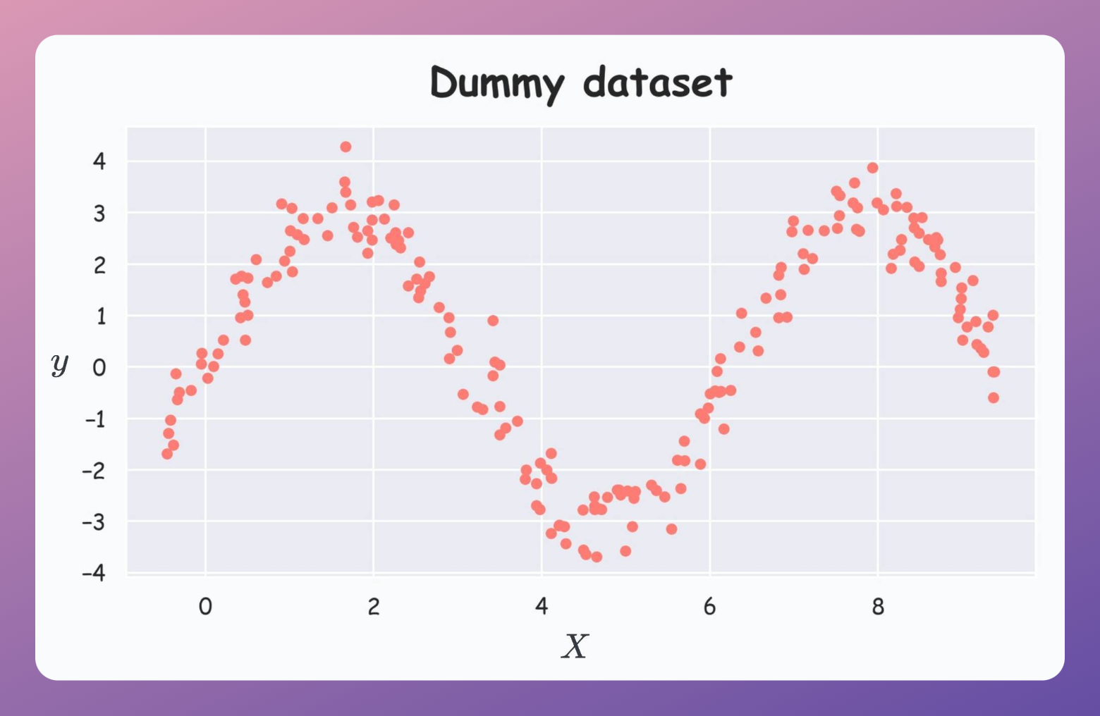
We construct the first tree on this dataset as follows:
Measuring the performance (R2), we get:
Now, we must construct the next tree. To do this, we fit another model on the residuals (true-predicted) of the first tree:
Yet again, we measure the performance of the current ensemble:
Tree1captures some variance, andtree2captures the residual left bytree1. So, the final prediction is the sum of both predictions.
The R2 score has jumped from 0.68 to 0.81.
Now, let’s construct another tree on the residuals (true-predicted) of the current ensemble:
Let’s measure the performance once again:
The R2 score has jumped from 0.81 to ~0.88.
We can continue to build the ensemble this way and generate better scores.
At this point, we can also visualize this performance improvement by incrementally plotting the fit obtained as we add more trees:
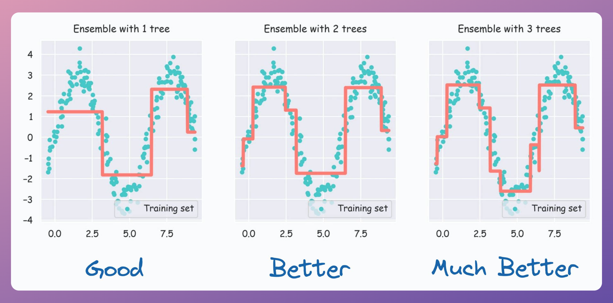
From the above diagram, it is clear that as we add more trees, the model tends to fit the dataset better.
And that is how Boosting is implemented. Now go back to the three variables we discussed above and noticed how we implemented our boosting model:
- How you construct each tree: Here, we relied on a decision tree's native tree construction strategy, which uses Gini impurity.
- How to construct the next tree based on the current trees: Here, we allowed the next model to learn the residuals left over by the previous models.
- How to weigh the contribution of each tree in the final model: Since the subsequent model learned the residuals and we were building a regression model, we added the output of all models to get the final regression output.
Simple, right?
And you'll be surprised that things we shall discuss ahead about XGBoost will make use of the exact same variables as well.
Let's dive in!
Formulating XGBoost
Consider a supervised learning problem. We would have a training dataset $D$ with a total number of samples $n$:

Assuming we are building a regression model just like we did in the demo above, we will have an ensemble of $K$ regression-based trees $f(x)$, whose output will be added to obtain the final output $F(x)$, as follows:
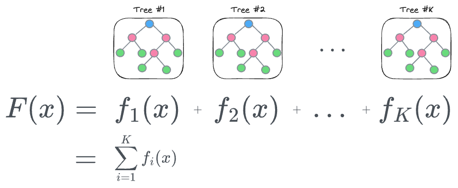
The next task is to train this model, and to do that, we must define a loss function, based on which the next tree will be created.
Now here's the thing with the demo we discussed earlier.
Since the subsequent model is trained on the residuals obtained from the current ensemble, the performance will always continue to improve and with sufficient number of trees, one can 100% overfit the dataset. A demo with 15 trees is shown below:
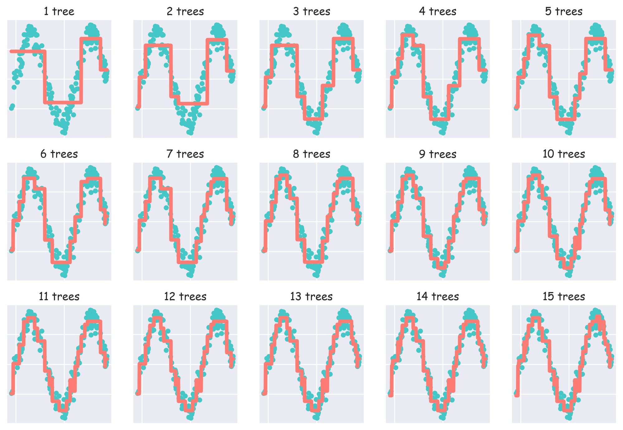
As a result, one can easily obtain an overly complex model even with sufficiently low number of trees in the ensemble.
While pruning techniques help, it is applied post-training to simplify a complex model. XGBoost’s researchers identified this as a problem and thought if it was possible to regularize tree models as they are being trained.
Thus, as far as I know, XGBoost was the first tree-based ensemble algorithm to introduce the idea of regularization in a tree.
More specifically, the idea is to define a loss function that minimizes both:
- the difference between the true prediction $y$ and the ensemble's prediction $F(x)$,
- the complexity of the model being training.
So, to begin this formulation, we can define a regularized cost function to train the model as follows:

- The first part (in green) computes the loss (error) over samples
- The second part (in blue) involves a cost applied on the tree models in the ensembles, which, ideally, should increase as the ensemble becomes complex.
Before we move ahead and define the ensemble's penalty, you must note that the regularization term in the cost function above is a part of the tree learning objective itself. It is not applied as an external hyperparameter which we typically define in tree-based models such as limiting the maximum depth of the tree or setting a cap on the maximum number of leaf nodes.
Moving on, it must be obvious to understand that the cost function $\mathcal{J}$ defined above cannot be optimized using traditional optimization methods such as gradient descent.
Thus, we must find ways to train it in a greedy stepwise manner, by adding one new tree at a time.
Recall that in our regression problem, the output computed after the $k^{th}$ iteration can be defined as follows:
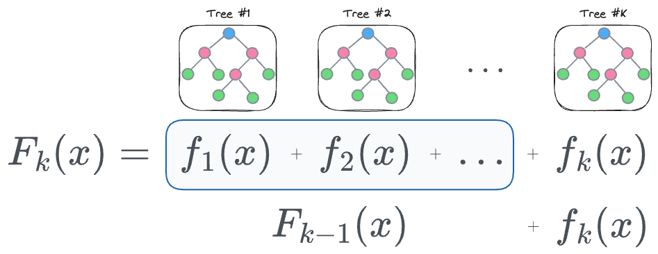
More formally, the output with $k$ trees is the same as the sum of output with $(k-1)$ trees and the $k^{th}$ tree, as defined below:

We can substitute this back into the cost function we defined above to get the following:
Read the full article
Sign up now to read the full article and get access to all articles for paying subscribers only.
Join today!

