The Probabilistic Origin of Regularization

👉

One of the major aspects of training any reliable ML model is avoiding overfitting.

In a gist, overfitting occurs when a model learns to perform exceptionally well on the training data.

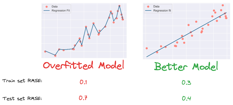
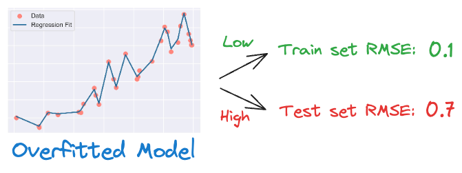
This may happen because the model is trying too hard to capture all unrelated and random noise in our training dataset, as shown below:

In this context, noise refers to any random fluctuations or inconsistencies that might be present in the data.

While learning this noise leads to a lower train set error and lets your model capture more intricate patterns in the training set, it comes at the tremendous cost of poor generalization on unseen data.

Metrics of an overfitted model. Low training error and high test error.

One of the most common techniques used to avoid overfitting is regularization.

Simply put, the core objective of regularization is to penalize the model for its complexity.

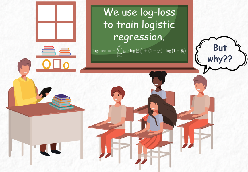
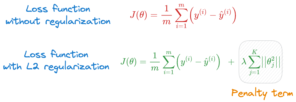
And if you have taken any ML course or read any tutorials about this, the most common they teach is to add a penalty (or regularization) term to the cost function, as shown below:

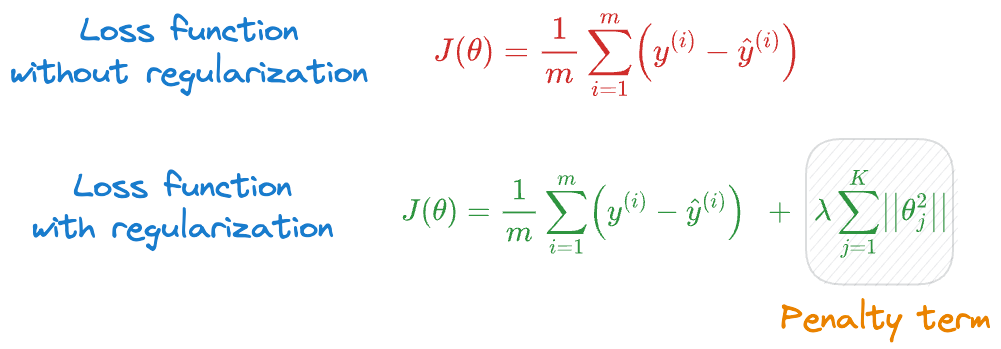
In the above expressions:

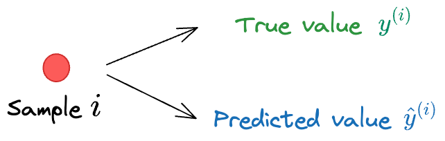
$y^{(i)}$ is the true value corresponding to sample $i$.
$\hat y^{(i)}$ is the model’s prediction corresponding to sample $i$, which is dependent on the parameters $(\theta_1, \theta_2, \cdots, \theta_K)$.

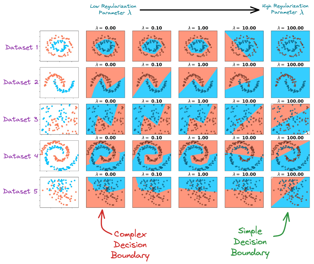
While we can indeed validate the effectiveness of regularization experimentally (as shown below), it’s worth questioning the origin of the regularization term from a probabilistic perspective.

Regularization experiment. Increasing the regularization parameter $\lambda$ creates simpler decision boundaries

More specifically:

Where did this regularization term originate from?
What does the regularization term precisely measure?
What real-life analogy can we connect it to?
Why do we add this regularization term to the loss?
Why do we square the parameters (specific to L2 regularization)? Why not any other power?
Is there any probabilistic evidence that justifies the effectiveness of regularization?

Turns out, there is a concrete probabilistic justification for regularization.

Yet, in my experience, most tutorials never bother to cover it, and readers are always expected to embrace these notions as a given.

Thus, this article intends to highlight the origin of regularization purely from a probabilistic perspective and provide a derivation that makes total logical and intuitive sense.

Let’s begin!

Maximum Likelihood Estimation (MLE)

Before understanding the origin of the regularization term, it is immensely crucial to learn a common technique to model labeled data in machine learning.

It’s called the maximum likelihood estimation (MLE).

We covered this in the following article, but let’s do it again in more detail.

Essentially, whenever we model data, the model is instructed to maximize the likelihood of observing the given data $(X,y)$.

More formally, a model attempts to find a specific set of parameters $\theta$ (also called model weights), which maximizes the following function:

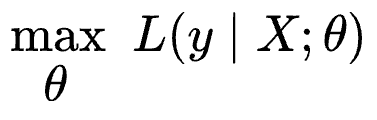
The above function $L$ is called the likelihood function, and in simple words, the above expression says that:

maximize the likelihood of observing $y$
given $X$
when the prediction is parameterized by some parameters $\theta$ (also called weights)

When we begin modeling:

We know $X$.
We also know $y$.
The only unknown is $\theta$, which we are trying to figure out.

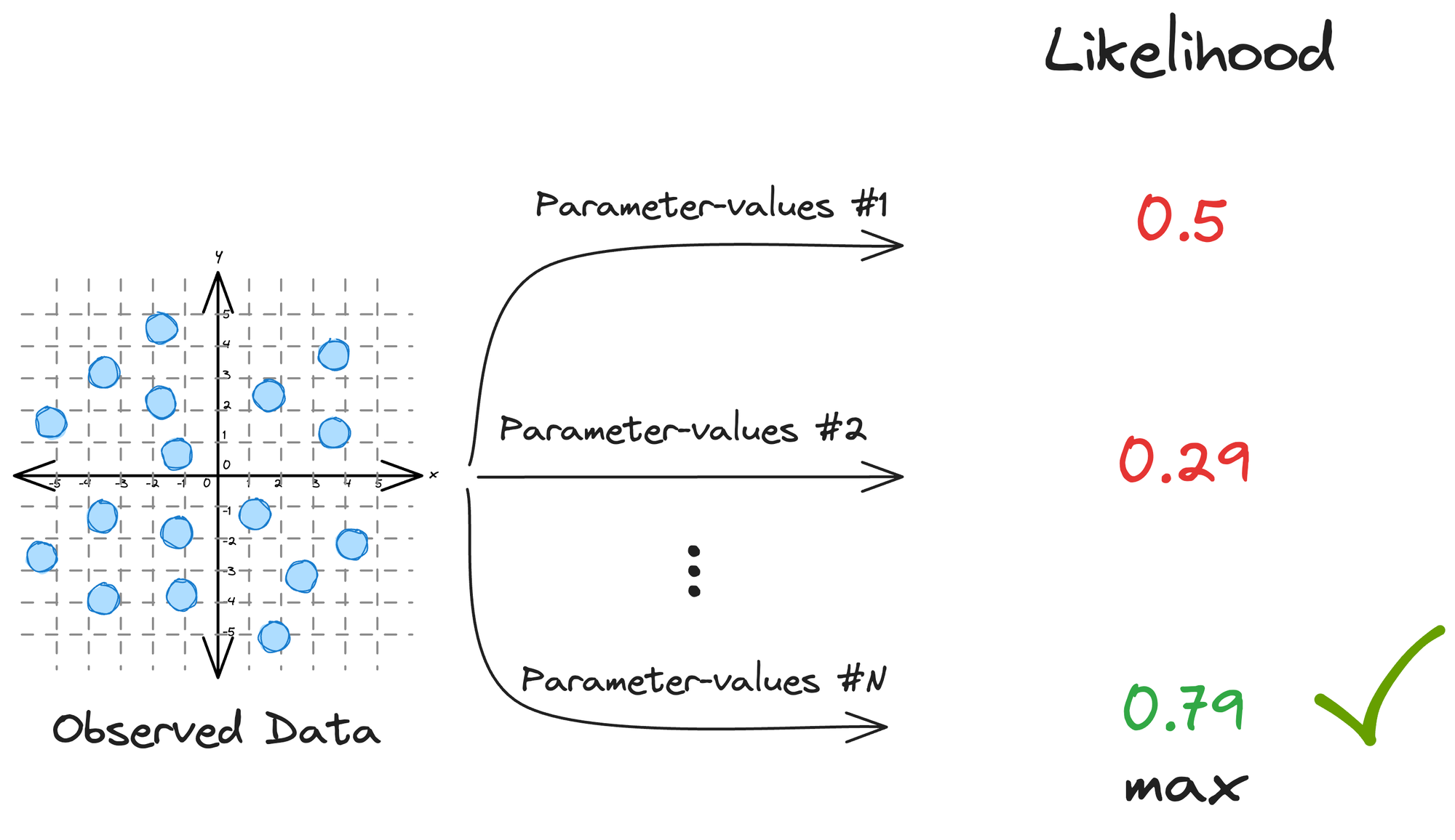
Thus, the objective is to find the specific set of parameters $\theta$ that maximizes the likelihood of observing the data $(X,y)$.

This is commonly referred to as maximum likelihood estimation (MLE) in machine learning.

MLE is a method for estimating the parameters of a statistical model by maximizing the likelihood of the observed data.

*MLE in one line: Find the parameter values that maximize the likelihood of data*

It is a common approach for parameter estimation in various regression models.

Let’s understand it with the help of an example.

An intuitive example of MLE

Imagine you walk into a kitchen and notice several broken eggshells on the floor.

Here’s a question: “Which of these three events is more likely to have caused plenty of eggshells on the floor?”

Someone was experimenting with them.
Someone was baking a cake.
Someone was creating an art piece with them.

Which one do you think was more likely to have happened?

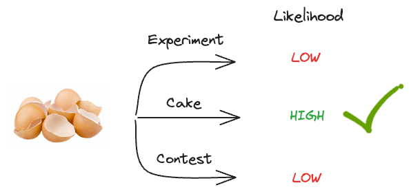
Let’s look at what could have led to eggshells on the floor with the highest likelihood.

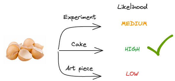
Likelihood of getting eggshells based on certain events

The likelihood of:

Conducting a science experiment that led to eggshells on the floor is MEDIUM.
Baking a cake that led to eggshells on the floor is HIGH.
Creating an art piece that led to eggshells on the floor is LOW.

Here, we’re going to go with the event with the highest likelihood, and that’s “baking a cake.”

Thus, we infer that the most likely thing that happened was that someone was baking a cake.

What we did was that we maximized the conditional probability of the event, given an explanation.

The event is what we observed, i.e., eggshells on the floor.
The “explanation,” as the name suggests, is the possible cause we came up with.

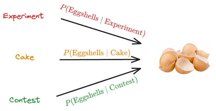
We did this because there’s a probability of:

“Eggshells” given “Experiment”
“Eggshells” given “Cake”
“Eggshells” given “Art piece”

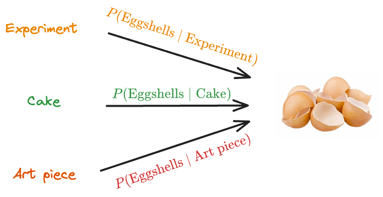
The conditional probability of getting eggshells given a certain event took place

We picked the one with the highest conditional probability $P(event|explanation)$.

Simply put, we tried to find the scenario that most likely led to the eggshells on the floor. This is called maximum likelihood.

This is precisely what we do in machine learning at times. We have a bunch of data and several models that could have generated that data.

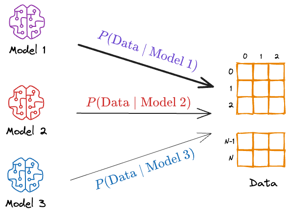
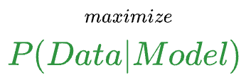
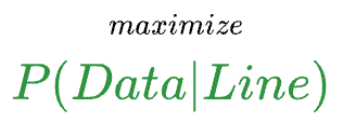
The conditional probability of observing the data given a model

First, we estimate the probability of seeing the data given “Model 1”, “Model 2”, and so on. Next, we pick the model that most likely produced the data.

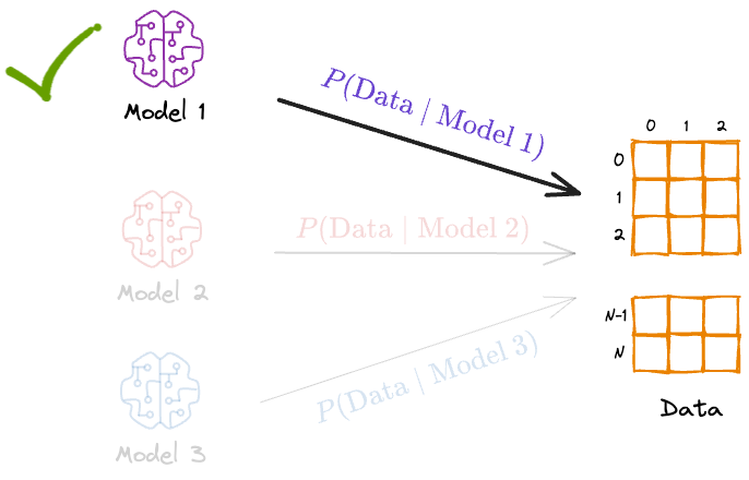
Selecting the model which generates the data with the highest likelihood

In other words, we’re maximizing the probability of the data given model.

MLE for linear regression

Next, let’s consider an example of using MLE for simple linear regression.

Consider we have the following data:

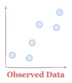
The candidate models that could have generated the above data our:

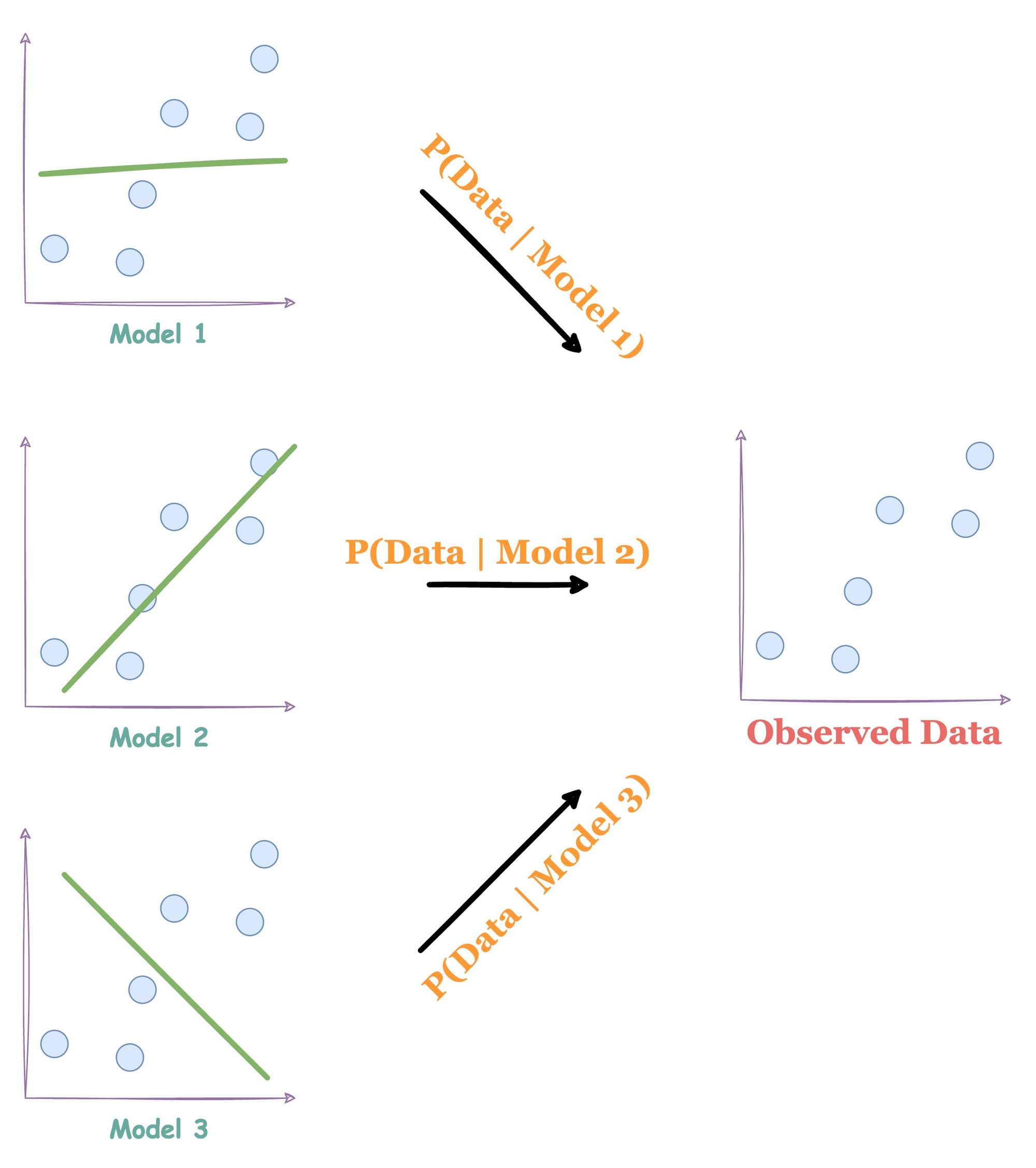
Three models that could have generated the observed data

It’s easy to figure out that Model 2 would have most likely generated the above data.

But how does a line generate points?

Let’s understand this specific to linear regression.

We also discussed this more from a technical perspective in the linear regression assumptions article, but let’s understand visually this time.

Consider the diagram below.

Say you have the line shown in Step 1, and you select data points on this line.

Recalling the data generation process from the above article, we discussed that linear regression generates data from a Gaussian distribution with equal variance.

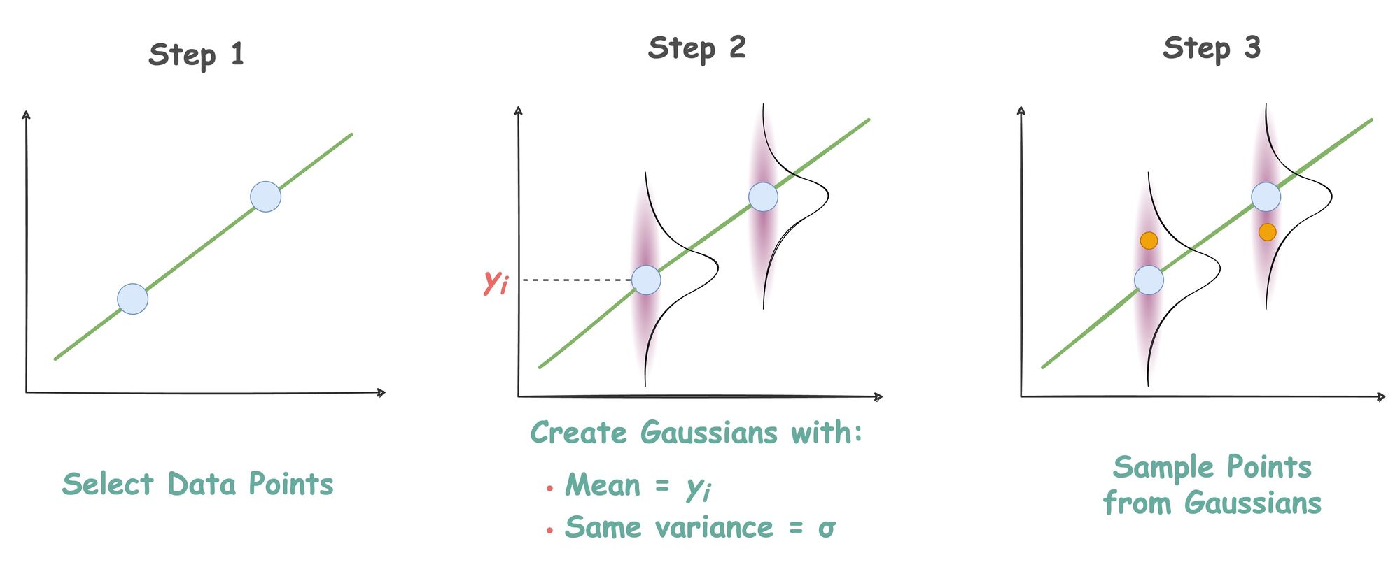
Generating data points from a line by sampling data from Gaussians

Thus, in step 2, we create Gaussians with equal variance centered at those points.

Lastly, in step 3, we sample points from these Gaussians.

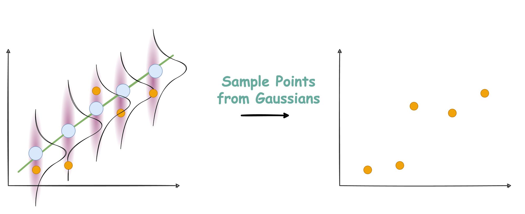
And that is how a line generates data points.

Now, in reality, we never get to see the line that produced the data. Instead, it’s the data points that we observe.

Thus, the objective boils down to finding the line that most likely produced these points.

We can formulate this as a maximum likelihood estimation problem by maximizing the likelihood of generating the data points given a model (or line).

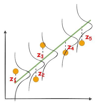
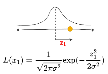
Distance of sampled points from the line

Let’s look at the likelihood of generating a specific point from a Gaussian:

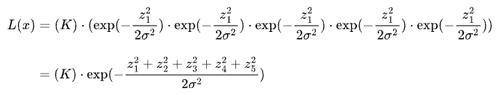
Similarly, we can write the likelihood of generating the entire data as the product of individual likelihoods:

Substitution the likelihood values from the Gaussian distribution, we get:

$K$ represents the constant obtained after multiplying the terms $\frac{1}{\sqrt{2\pi\sigma^2} }$

Maximizing the above expression is the same as minimizing the squared sum term in the exponent.

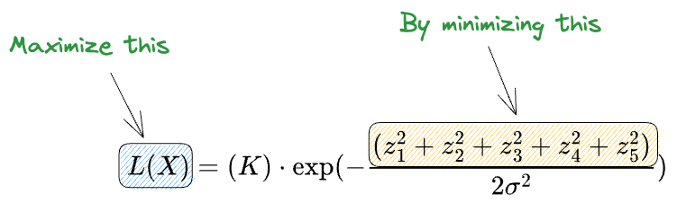
And this is precisely the least squares error.

Linear regression finds the line that minimizes the sum of squared distances.

This proves that finding the line that most likely produces a point using maximum likelihood is exactly the same as minimizing the least square error using linear regression.

The Origin of Regularization

So far, we have learned how we estimate the parameters using maximum likelihood estimation.

We also looked at the example of eggshells, and it helped us intuitively understand what MLE is all about.

Let’s recall it.

The intuition to regularization

This time, let’s replace “Art piece” with an “Eggshell throwing contest.”

So yet again, we have three possibilities that may have led to the observed event.

Someone was experimenting with them.
Someone was baking a cake.
Someone was playing an Eggshell throwing contest.

Which one do you think was more likely to have happened?

It’s obvious that baking a cake will still lead to eggshells with a high probability.

But an Eggshell throwing contest will create eggshells on the floor with a very high probability.

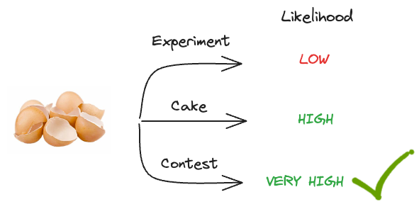
Contest has a higher likelihood of generating the evidence

It’s certain that an eggshell-throwing contest will lead to eggshells on the floor.

However, something tells us that baking a cake is still more likely to have happened and not the contest, isn’t it?

One reason is that an eggs-throwing contest is not very likely – it’s an improbable event.

Thus, even though it’s more likely to have generated the evidence, it’s less likely to have happened in the first place. This means we should still declare “baking a cake” as the more likely event.

But what makes us believe that baking a cake is still more likely to have produced the evidence?

It’s regularization.

In this context, regularization lets us add an extra penalty, which quantifies the probability of the event itself.

Even though our contest will undoubtedly produce the evidence, it is not very likely to have happened in the first place.

This lets us still overweigh “baking a cake” and select it as the most likely event.

This is the intuition behind regularization.

Now, at this point, we haven’t yet understood the origin of the regularization term.

But we are not yet close to understanding its mathematical formulation.

Specifically talking about L2 regularization, there are a few questions that we need to answer:

Where did the squared term come from?
What does this term measure probabilistically?
How can we be sure that the term we typically add is indeed the penalty term that makes the most probabilistic sense?

The same can be translated to L1 regularization as well.

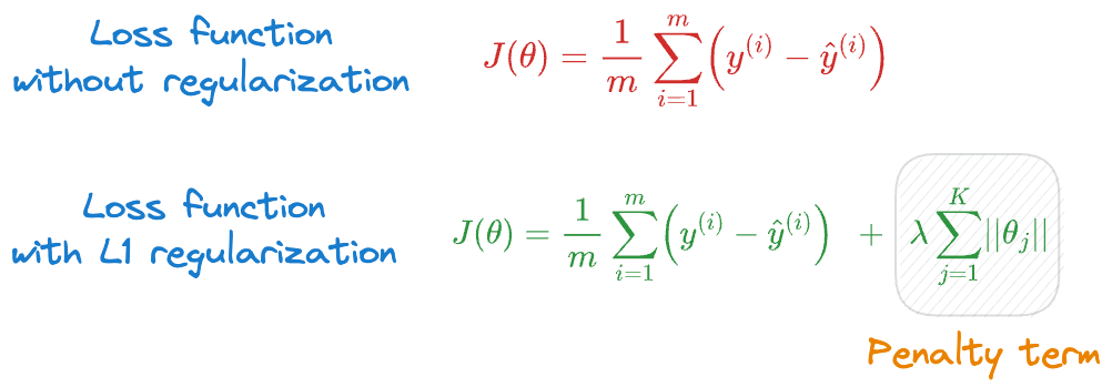
Where did the absolute sum of parameters come from?
What does this term measure probabilistically?
How can we be sure that the term we typically add is indeed the penalty term that makes the most probabilistic sense?

Let’s delve into the mathematics of regularization now.