A Crash Course of Model Calibration – Part 2

In the first part of the model calibration deep dive, we went into quite a lot of detail about the core idea behind this topic, defining calibration and techniques to measure the extent of miscalibration in machine learning models.

A Crash Course of Model Calibration – Part 1

How to make ML models reflect true probabilities in their predictions?

Daily Dose of Data ScienceAvi Chawla

Moreover, we also understood some historical background about how models have evolved to become increasingly miscalibrated.

This is part 2, where we shall dive into some limitations of the methods we discussed in part 1, and also discuss some common techniques to calibrate machine learning models.

Quick recap

To recap, consider the following plot again, which compares a LeNet (developed in 1998) with a ResNet (developed in 2016) on the CIFAR-100 dataset.

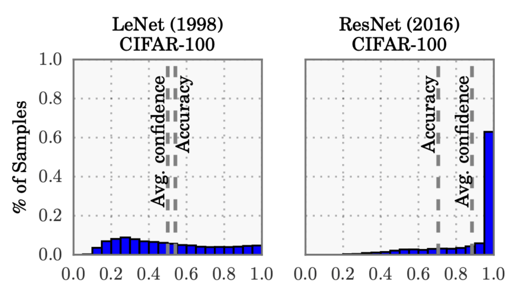
From the above plot, it is clear that:

• The average confidence of LeNet (an old model) closely matches its accuracy.
• In contrast, the average confidence of the ResNet (a relatively modern model) is substantially higher than its accuracy.

Thus, we can see that the LeNet model is well-calibrated since its confidence closely matches the expected accuracy. However, the ResNet’s accuracy is better $(0.7>0.5)$, but the accuracy does not match its confidence.

To put it another way, it means that the ResNet model, despite being more accurate overall, is overconfident in its predictions. So, while LeNet's average confidence aligns well with its actual performance, indicating good calibration, ResNet's higher average confidence compared to its accuracy shows that it often predicts outcomes with higher certainty than warranted.

Why does this happen?

In Part 1, we also discussed some technical reasons (training procedure-related) for miscalibration that helped us understand why modern models miscalibrate more, etc.

Why calibration is important?

One question that typically comes up at this stage is:

Why do we care about calibrating models, especially when we are able to build more accurate systems?

The motivation is quite similar to what we also discussed in the conformal prediction deep dive linked below:

Conformal Predictions: Build Confidence in Your ML Model’s Predictions

A critical step towards building and using ML models reliably.

Daily Dose of Data ScienceAvi Chawla

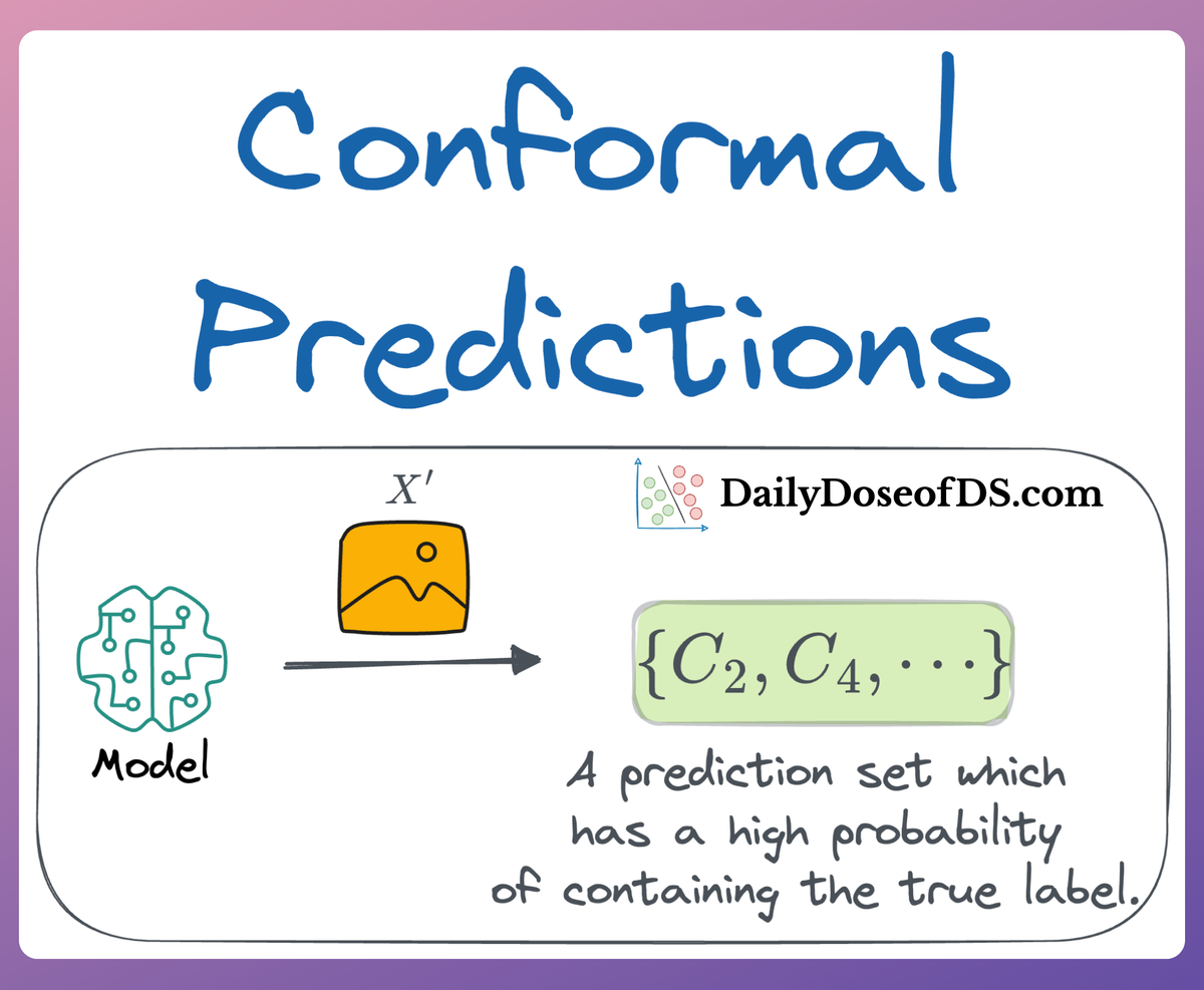
Blindly trusting an ML model’s predictions can be fatal at times, especially in high-stakes environments where decisions based on these predictions can affect human lives, financial stability, or critical infrastructure.

While an accuracy of “95%” looks good on paper, the model will never tell you which specific 5% of its predictions are incorrect when used in downstream tasks.

To put it another way, although we may know that the model’s predictions are generally correct a certain percentage of the time, the model typically cannot tell much about a specific prediction.

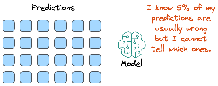
As a result, in high-risk situations like medical diagnostics, for instance, blindly trusting every prediction can result in severe health outcomes.

Thus, to mitigate such risks, it is essential to not only solely rely on the predictions but also understand and quantify the uncertainty associated with these predictions.

But given that modern models are turning out to be overly confident in their predictions (which we also saw above), it is important to ensure that our model isn't one of them.

Such overconfidence can be problematic, especially in applications where the predicted probabilities are used to make critical decisions.

For instance, consider automated medical diagnostics once again. In such cases, control should be passed on to human doctors when the model's confidence of a disease diagnosis network is low.

More specifically, a network should provide a calibrated confidence measure in addition to its prediction. In other words, the probability associated with the predicted class label should reflect its ground truth correctness likelihood.

And this is not just about communicating the true confidence. Calibrated confidence estimates are also crucial for model interpretability.

Humans have a natural cognitive intuition towards probabilities. Good confidence estimates provide a valuable extra bit of information to establish trustworthiness with the user – especially for neural networks, whose classification decisions are often difficult to interpret.

But if we don't have any way to truly understand the model's confidence, then an accurate prediction and a guess can look the same.

Lastly, in many complex machine learning systems, models depend on each other and can also interact with each other. Single classifiers are often inputs into larger systems that make the final decisions.

If the models are calibrated, it simplifies interaction. Calibration allows each model to focus on estimating its particular probabilities as well as possible. And since the interpretation is stable, other system components don’t need to shift whenever models change.

Reliability diagrams

Reliability Diagrams are a visual way to inspect how well the model is currently calibrated. More specifically, this diagram plots the expected sample accuracy as a function of the corresponding confidence value (softmax) output by the model.

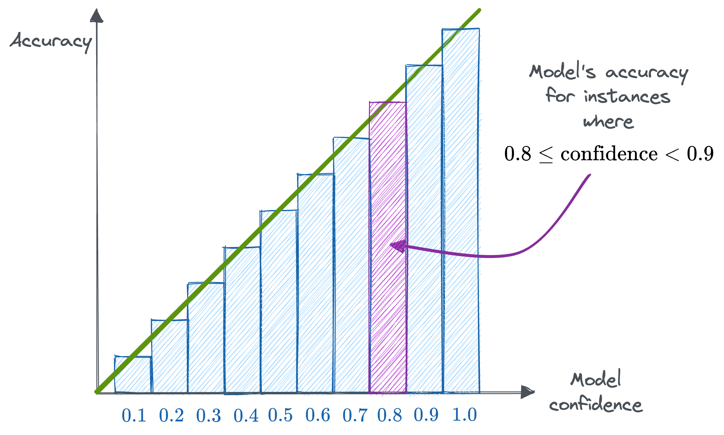
If the model is perfectly calibrated, then the diagram should plot the identity function as depicted above.

To estimate the expected accuracy, we group predictions into $M$ interval bins each of size $\frac{1}{M}$ (as shown above) and calculate the accuracy of each bin.

Let $B_m$ be the set of instances whose confidence values fall into the corresponding interval. Then, the accuracy of the model for those predictions is given by:

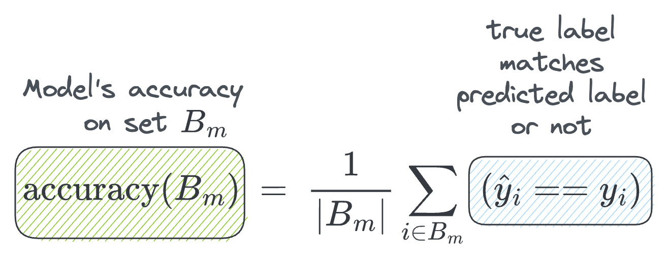
• where $\hat {y_i}$ is the predicted class for sample $i$.
• $y_i$ is the true class label for sample $i$.

Next, we can define the average confidence within bin $B_m$ as follows:

• where $\hat p_i$ is the confidence outputted by the model on sample $i$.

Quite intuitively, for a perfectly calibrated model, we will have $\text{accuracy}(B_m) = \text{confidence}(B_m)$ for all $m \in \{1, 2, \cdots, M\}$.

Expected Calibration Error (ECE)

Reliability diagrams are an extremely useful tool to visually assess whether a model is well-calibrated or not. In fact, it can also tell specific confidence values where the model is underestimating/overestimating, and we can then inspect those instances if possible.

That said, it is often also useful to compute a scalar value that measures the amount of miscalibration.

One way to approximate the expected calibration error shown above is by partitioning predictions into $M$ equally-spaced bins (similar to what we saw in the reliability diagrams above) and taking a weighted average of the bins’ accuracy/confidence difference. This is denoted below:

• where $n$ is the total number of samples.
• $|B_m|$ is the size of the set of instances whose confidence falls in the divided range.

For more details about ECE, you can read part 1:

A Crash Course of Model Calibration – Part 1

How to make ML models reflect true probabilities in their predictions?

Daily Dose of Data ScienceAvi Chawla

Calibration methods

In this section, we shall discuss some post-processing methods that help us produce calibrated probabilities.

To do so, each method requires a hold-out validation set, which, in practice, can be the same set used for hyperparameter tuning at the time of model training.

Binary classification models

First, let's discuss calibration in the binary setting $(y_i = \{0, 1\})$.