Where Did The Assumptions of Linear Regression Originate From?
The most extensive and in-depth guide to linear regression.
Introduction
The first algorithm that every machine learning course teaches is linear regression.
It’s undoubtedly one of the most fundamental and widely used algorithms in statistics and machine learning.
This is primarily because of its simplicity and ease of interpretation.
However, despite its prevalence, there is often a surprising oversight – understanding the assumptions that ensure the effectiveness of linear regression.
In other words, linear regression is only effective when certain assumptions are validated. We must revisit the model (or data) if the assumptions are violated.
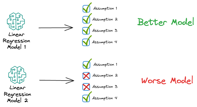
In my experience, when someone first learns linear regression, either of the two things happens:
- The teaching material does not highlight the critical assumptions that go into linear regression, which guarantees it to work effectively.
- Even if it does, in most cases, folks are never taught about the origin of those assumptions.
But it is worth questioning the underlying assumptions of using a specific learning algorithm and why those assumptions should not be violated.
In other words, have you ever wondered what is the origin of linear regression's assumptions?
They can't just appear from thin air, can they?
There should be some concrete reasoning to support them, right?
Thus, in this blog, let me walk you through the origin of each of the assumptions of linear regression in detail.
We will learn the following:
- A quick overview of Linear Regression.
- Why we use Mean Squared Error in linear regression – from a purely statistical perspective.
- The assumed data generation process of linear regression.
- The critical assumptions of Linear Regression.
- Why these assumptions are essential.
- How these assumptions are derived.
- How to validate them.
- Measures we can take if the assumptions are violated.
Let's begin!
Linear Regression (A quick walkthrough)
Linear regression models a linear relationship between the features $(X)$ and the true/observed output variable $(y)$.
The estimate $\hat y $ is written as:
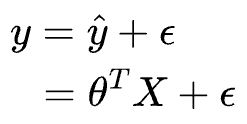
Where:
- $y$ is the observed/true dependent variable.
- $\hat y$ is the modeled output.
- $X$ represents the independent variables (or features).
- $\theta$ is the estimated coefficient of the model.
- $\epsilon$ is the random noise in the output variable. This accounts for the variability in the data that is not explained by the linear relationship.
The primary objective of linear regression is to estimate the values of $\theta = (\theta_{1}, \theta_{2}, \cdots, \theta_{n})$ that most closely estimate the observed dependent variable $y$.
What do we minimize and why?
Once we have formulated the model, it's time to train it. But how do we learn the parameters?
Everyone knows we use the mean squared loss function.
But why this function? Why not any other function?
Let's understand.
As discussed above, we predict our target variable $y$ using the inputs $X$ as follows (subscript $i$ is the index of the data point):

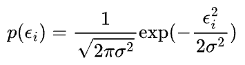
Here, $\Large \epsilon_{i}$ is an error term that captures the unmodeled noise for a specific data point ($i$).
We assume the noise is drawn from a Gaussian distribution with zero mean based on the central limit theorem (there's more on why we assume Gaussian noise soon).
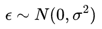
Thus, the probability of observing the error term can be written as:
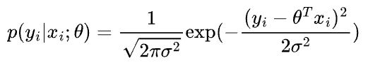
We call this the distribution of $y$ given $x$ parametrized by $\theta$. We are not conditioning on $\theta$ because it’s not a random variable.
Instead, for a specific set of parameters, the above tells us the probability of observing the given data point $i$.
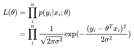
Next, we define the likelihood as:
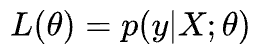
The likelihood is a function of $\theta$. It means that by varying $\theta$, we can fit a distribution to the observed data.
Finding the best fit is called maximum likelihood estimation (MLE).
We further write it as a product for individual data points in the following form because we assume independent observations.
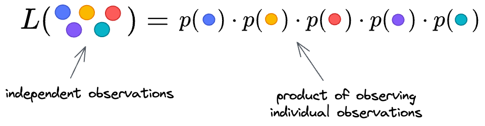
Thus, we get:
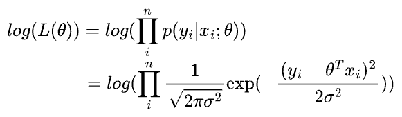
Since the log transformation is monotonic, we use the log-likelihood below to optimize MLE.
Simplifying, we get:
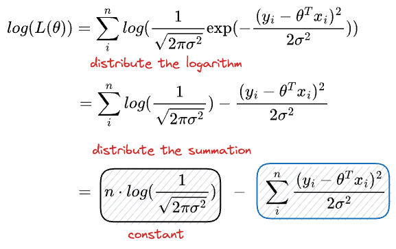
To find the best Gaussian that describes the true underlying model which generates our data, in other words, the best θ, we need to find the parameters that maximizes the log-likelihood.
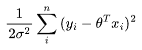
Maximizing the above expression is equivalent to minimizing the second term.
And if you notice closely, it's precisely the least squares.
And this is the origin of least-squares in linear regression and that's why we fit a linear regression model using least-squares.
Now recall the faulty reasoning we commonly hear about minimizing least-squares.
- Some justify it by saying that squared error is differentiable, which is why we use it. WRONG.
- Some compare it to absolute loss and say that squared error penalizes large errors. WRONG.
Each of these explanations is incorrect and flawed.
Instead, there's a clear reasoning behind why using least-squares gives us the optimal solution.
To summarize, linear regression tries to find the best model in the form of a linear predictor plus a Gaussian noise term that maximizes the probability of drawing our data from it.
And for the probability of observing the data to be maximum, least squares should be minimum:
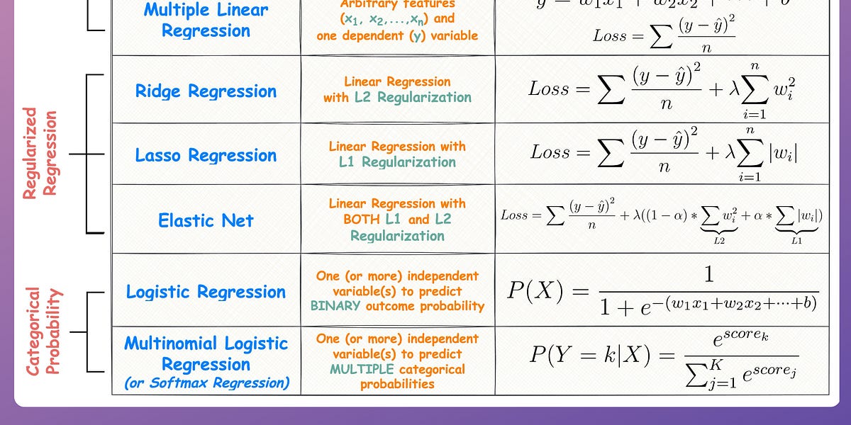
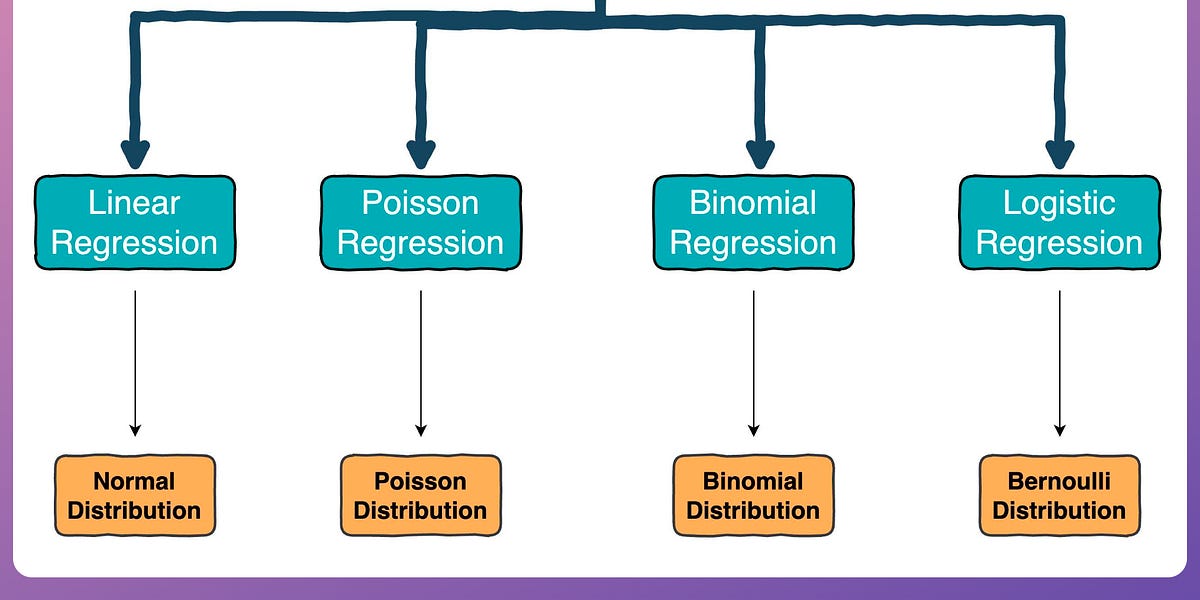
Common variations of linear regression
Linear regression has many variations, as summarized below:
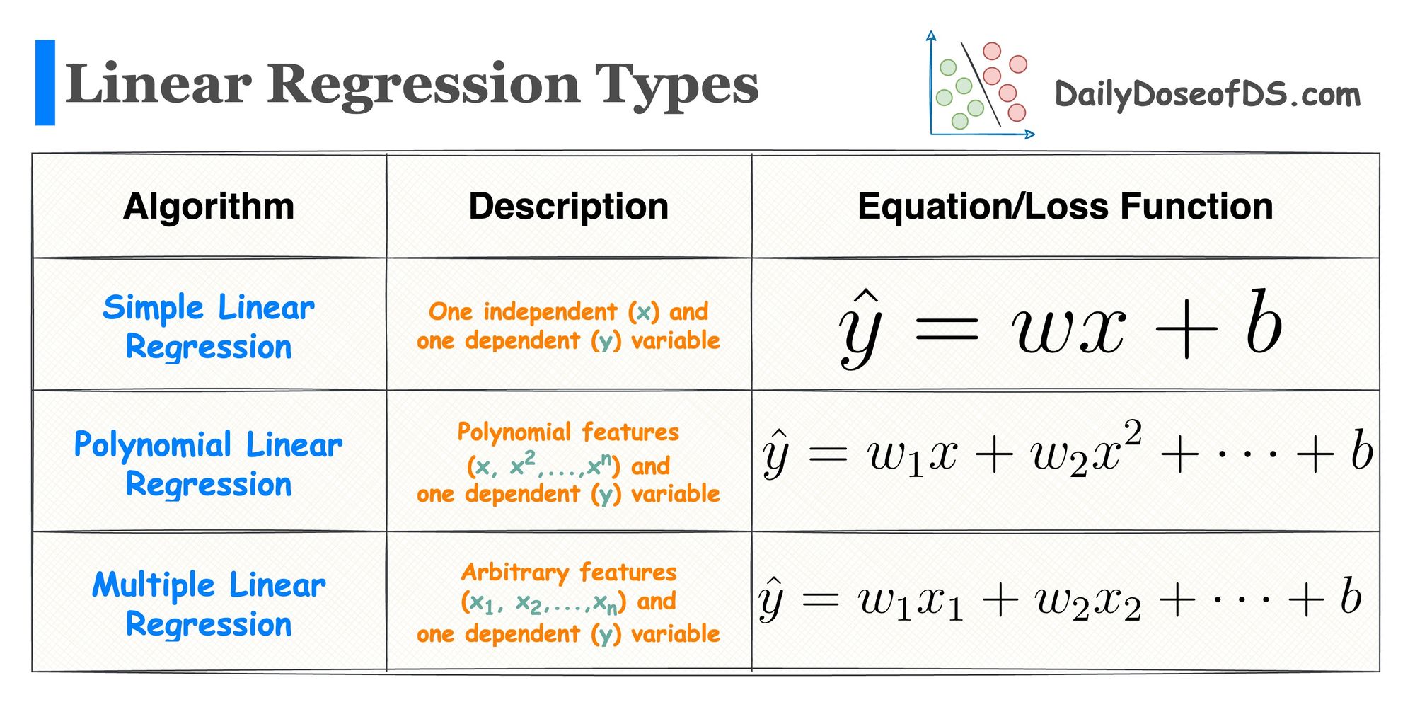
We have already covered them in detail below:
Assumptions of linear regression
We'll derive them pretty soon. But for now, let's learn what they are.
Also, we'll derive them from scratch, i.e., without having any prior information that these assumptions even exist.
Assumption #1: Linearity
This is the most apparent assumption in linear regression.

If you model the dependent variable $(y)$ as a linear combination of independent variables $(X)$, you inherently assume it is true and viable.
Assumption #2: Normal distribution of error
The second assumption of linear regression is that the error terms $\epsilon$ follow a normal distribution.
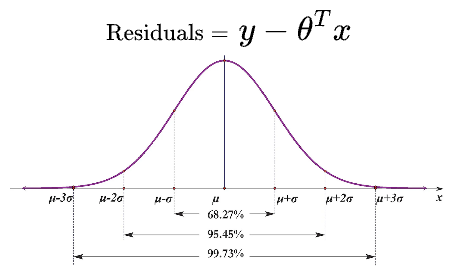
When the residuals are normally distributed, it enables more robust statistical inference, hypothesis testing, and constructing more reliable confidence intervals.
Departure from normality can lead to misleading conclusions and affect the validity of statistical tests.
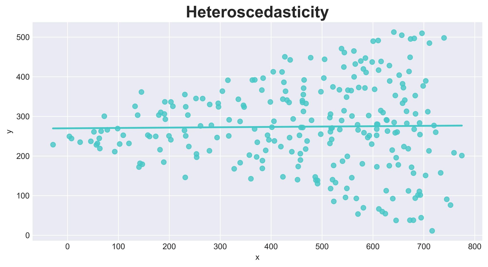
Assumption #3: Homoscedasticity
The third assumption is homoscedasticity, which refers to the constant variance of the error term $\epsilon$ across all levels of the independent variable(s).
In other words, the spread of the residuals should be consistent along the regression line.
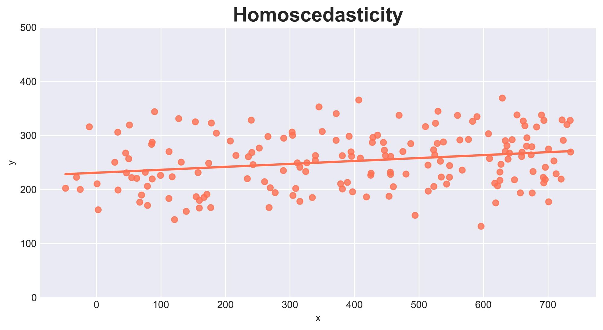
If the assumption is violated and the error term's variability changes with the predicted values, it is known as Heteroscedasticity, which can lead to biased and inefficient estimates.
Assumption #4: No Autocorrelation
The fourth assumption of linear regression is the independence of errors.
Simply put, the absence of autocorrelation implies that each data point's error terms (residuals) are not correlated with the error terms of other data points in the dataset.
Violating this assumption leads to autocorrelation, where the errors are correlated across observations, affecting the model's accuracy and reliability.
Assumption #5: No Multicollinearity (Additional Assumption)
Although not listed in the initial assumptions, Multicollinearity is another important consideration in multiple linear regression, where two or more independent variables are highly correlated.
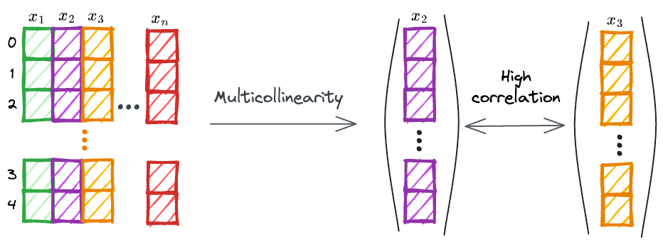
Multicollinearity can also arise if an independent variable can be approximated as a linear combination of some other independent variables.
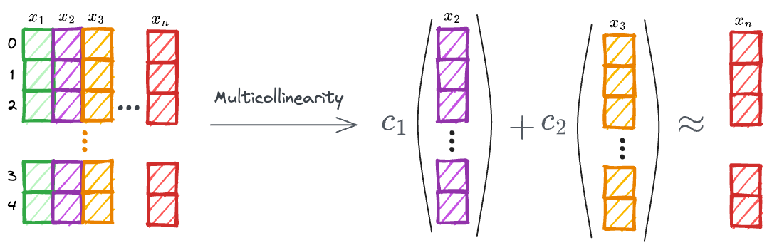
High Multicollinearity can cause numerical instability and make it challenging to interpret the individual effects of each independent variable.
The origin of assumptions
Now that we know the assumptions of linear regression, let's understand where these assumptions come from.
But from here, I want you to forget that these assumptions even exist.
See, any real answer should help you design the algorithm and derive these assumptions from scratch without knowing anything about them beforehand.
It is like replicating the exact thought process when a statistician first formulated the algorithm.
To understand this point better, ask yourself a couple of questions.
At the time of formulating the algorithm:
- Were they aware of the algorithm? NO.
- Were they aware of the assumptions that will eventually emerge from the algorithm? NO.
All they had was some observed data, which they wanted to model.
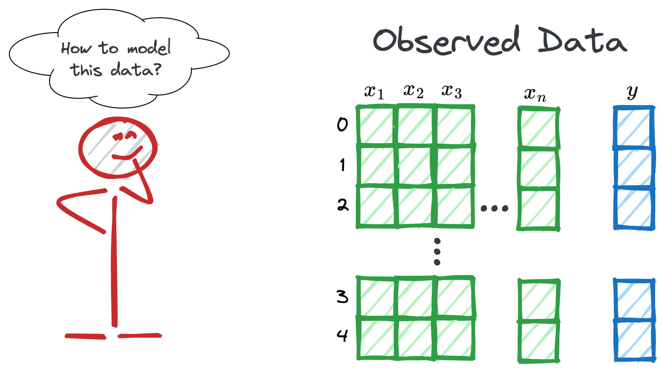
Thus, we should imitate that thought process too.
The assumed data generation process
Essentially, whenever we model a dataset, we think about the process that could have generated the observed data.
This is called the data generation process.
The data generation process for linear regression involves simulating a linear relationship between the dependent variable and one or more independent variables.
This process can be broken down into the following steps: