A Crash Course on Causality – Part 2

In the first part of the causality deep dive, we went into quite a lot of detail about the core idea behind this topic, why it is essential in business contexts, and some common techniques used in causal inference.

A Crash Course on Causality – Part 1

A guide to building robust decision-making systems in businesses with causal inference.

Daily Dose of Data ScienceAvi Chawla

We also spent some time understanding counterfactual learning and how it relates to causal scenarios.

This is part 2 of the causality deep dive and we will continue from where we ended part 1.

Quick recap

Towards the end of part 1, we discussed observational studies. As the name suggests, observational studies involve observing and analyzing existing data without manipulating the environment or conditions.

This approach allows researchers to study real-world scenarios where randomization is impossible or unethical.

However, there are usually many more differences between the observations in addition to the treatment that affects the outcome.

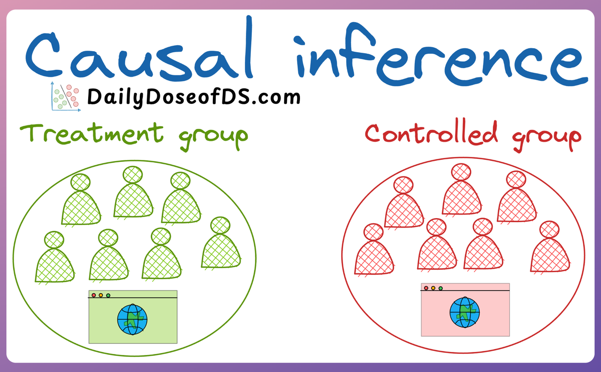
For instance, consider the marketing campaign example we discussed in part 1, where we determined its causal impact on sales.

In the earlier discussion, we only considered whether a person was shown the marketing campaign or not.

However, in real life, there will be various other factors that may potentially impact sales, such as the following:

• Customer Demographics: Age, gender, income level, and education can all influence purchasing behavior. Younger customers might respond differently to the campaign compared to older customers.
• Geographical Location: Customers from different regions might have varying levels of exposure to the campaign and different purchasing power. Cultural differences and local economic conditions can also play significant roles.
• Purchase History: Customers with a history of frequent purchases might react differently to the campaign compared to those who rarely buy. Their previous interactions with the brand can influence their responsiveness to marketing efforts.
• Economic Conditions: Broader economic factors, such as inflation rates, employment levels, and consumer confidence, can impact overall spending habits.
• And so on...

Let's assume that we have gathered data for all such potential factors and fit a regression model:

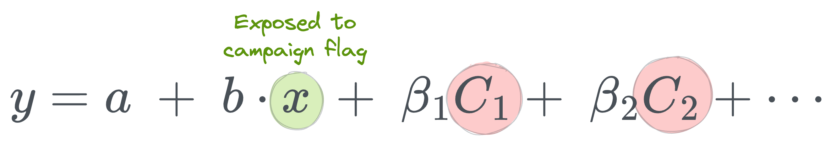
Here:

• $y$ is the outcome variable.
• $x$ is the treatment indicator.
• $a$ is the intercept.
• $b$ is the slope (causal effect of the treatment).
• $C_i$ is the control variable we discussed above, and $\beta_i$ is its coefficient in the regression model.

Unlike the RCT case, this time, we cannot confidently say that $b$ is the true causal impact of the marketing campaign on the outcome variable (sales).

This is primarily because we cannot control for every variable. Moreover, there are variables impacting sales that we don’t have data on, don’t know that they are important, or simply cannot measure (think about "customer preferences," "competitor actions," or "economic conditions").

This is commonly known as the Omitted Variable Bias in causality.

This is a serious problem because if we leave out important variables that ideally must be accounted for, the model attributes their impact to those variables we included in the study. This biases the estimate of the causal impact.

Okay, so what can we do to handle this?

Randomization has already been dismissed, and we have identified issues with observational study too.

Instrumental Variables

Introduction

An instrumental variable is a variable that is correlated with the treatment variable but not directly with the outcome variable, except through its effect on the treatment. This allows us to isolate the causal effect of the treatment on the outcome.

To use an instrumental variable, we follow a process called two-stage least squares (2SLS):

1. First Stage: Regress the treatment variable on the instrumental variable.
2. Second Stage: Use the predicted values from the first stage as the independent variable in a regression with the outcome variable.

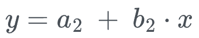
For example, if $z$ is our instrumental variable and $x$ is the treatment:

1. First stage:

2. Second stage:

While this requires us to fit two models, in practice, we do not need to do that.

This is because one can compute the coefficient of interest ($b_2$) or the causal impact of treatment $x$ on the outcome $y$ using the following closed-form solution:

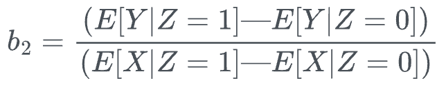
Yet again, we can use the same simple linear regression idea which we discussed in part 1.

First, we calculate the expected values and the coefficient $b_1$ in the first stage as follows:

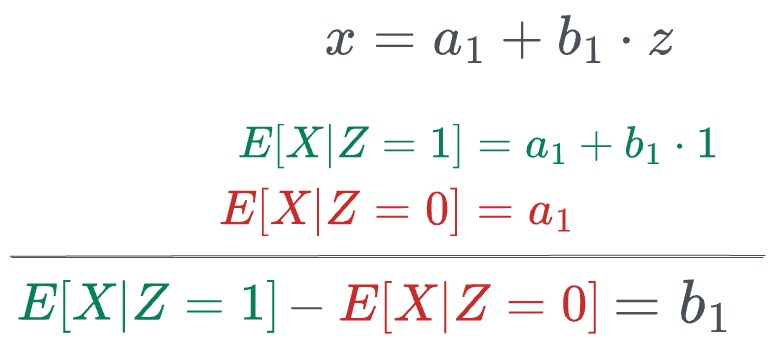
Next, we calculate the expected values and the coefficient $b_2$ in the second stage as follows. But before doing that, we substitute the value of $x$ in terms of $z$: