Why Bagging is So Ridiculously Effective At Variance Reduction?

Random forest is a pretty powerful and robust model, which is a combination of many different decision trees.

What makes them so powerful over a traditional decision tree model is Bagging:

Anyone who has ever heard of Random Forest has surely heard of Bagging and how it works.

This is because, in my experience, there are plenty of resources that neatly describe:

• How Bagging algorithmically works in random forests.
• Experimental demo on how Bagging reduces the overall variance (or overfitting).

However, these resources often struggle to provide an intuition on:

1. Why Bagging is so effective.
2. Why do we sample rows from the training dataset with replacement.
3. The mathematical demonstration that verifies variance reduction.

Thus, in this article, let me address all of these above questions and provide you with a clear and intuitive reasoning on:

• Why bagging makes the random forest algorithm so effective at variance reduction.
• Why does bagging involves sampling with replacement?
• How do we prove variance reduction mathematically?

Let’s begin!

The overfitting experiment

Decision trees are popular for their interpretability and simplicity.

Yet, unknown to many, they are pretty infamous when it comes to overfitting any data they are given.

This happens because a standard decision tree algorithm greedily selects the best split at each node, making its nodes more and more pure as we traverse down the tree.

Unless we don’t restrict its growth, nothing can stop a decision tree from 100% overfitting the training dataset.

For instance, consider that we have the following dummy data, and we intentionally want to 100% overfit it with, say, a linear regression model.

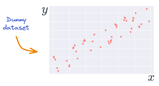
This task will demand some serious effort by the engineer.

In other words, we can’t just run linear_model.fit(X, y) in this case to directly overfit the dataset.

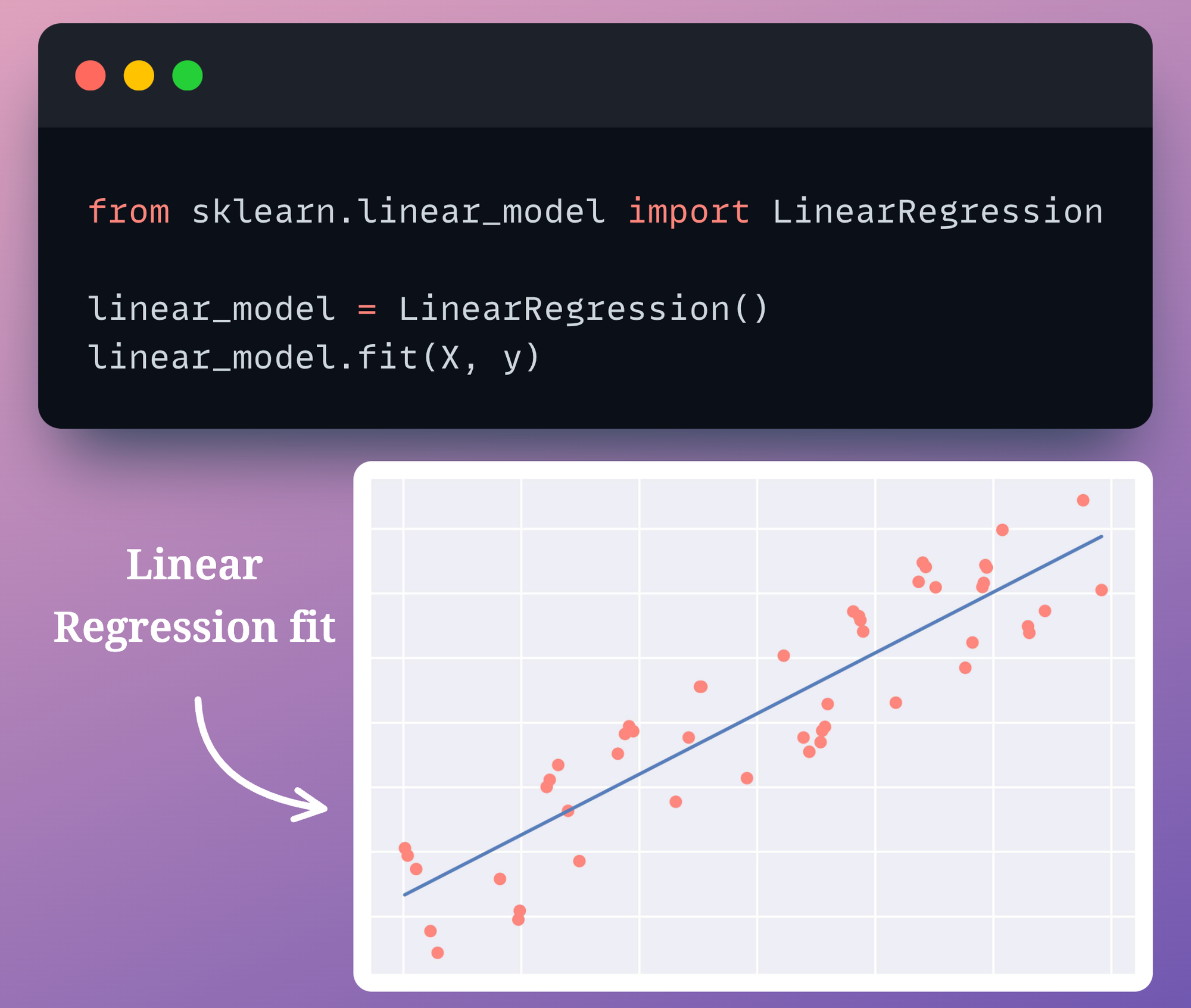
Instead, as mentioned above, this will require some serious feature engineering effort to entirely overfit the given dataset.

For instance, to intentionally overfit this dummy dataset, we would have to explicitly create relevant features, which, in this case, would mostly be higher-degree polynomial features.

This is shown below:

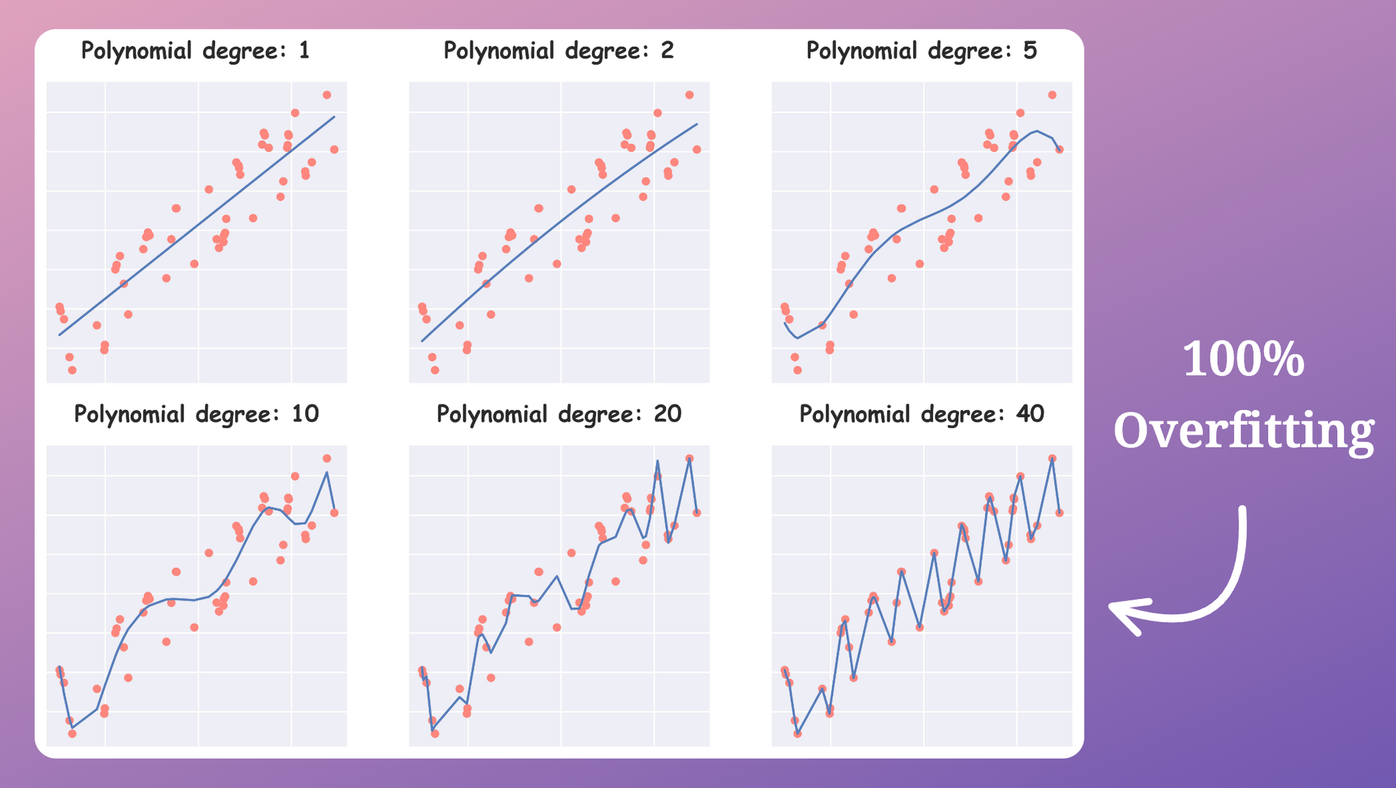
As shown above, as we increase the degree of our feature $x$ in our polynomial regression, the model starts to overfit the dataset more and more.

With a polynomial degree of $40$, the model entirely overfits the dataset.

The point is that overfitting this dataset (on any dataset, for that matter) with linear regression typically demands some engineering effort.

While the above dataset was easy to overfit, a complex dataset with all sorts of feature types may require serious effort to intentionally overfit the data.

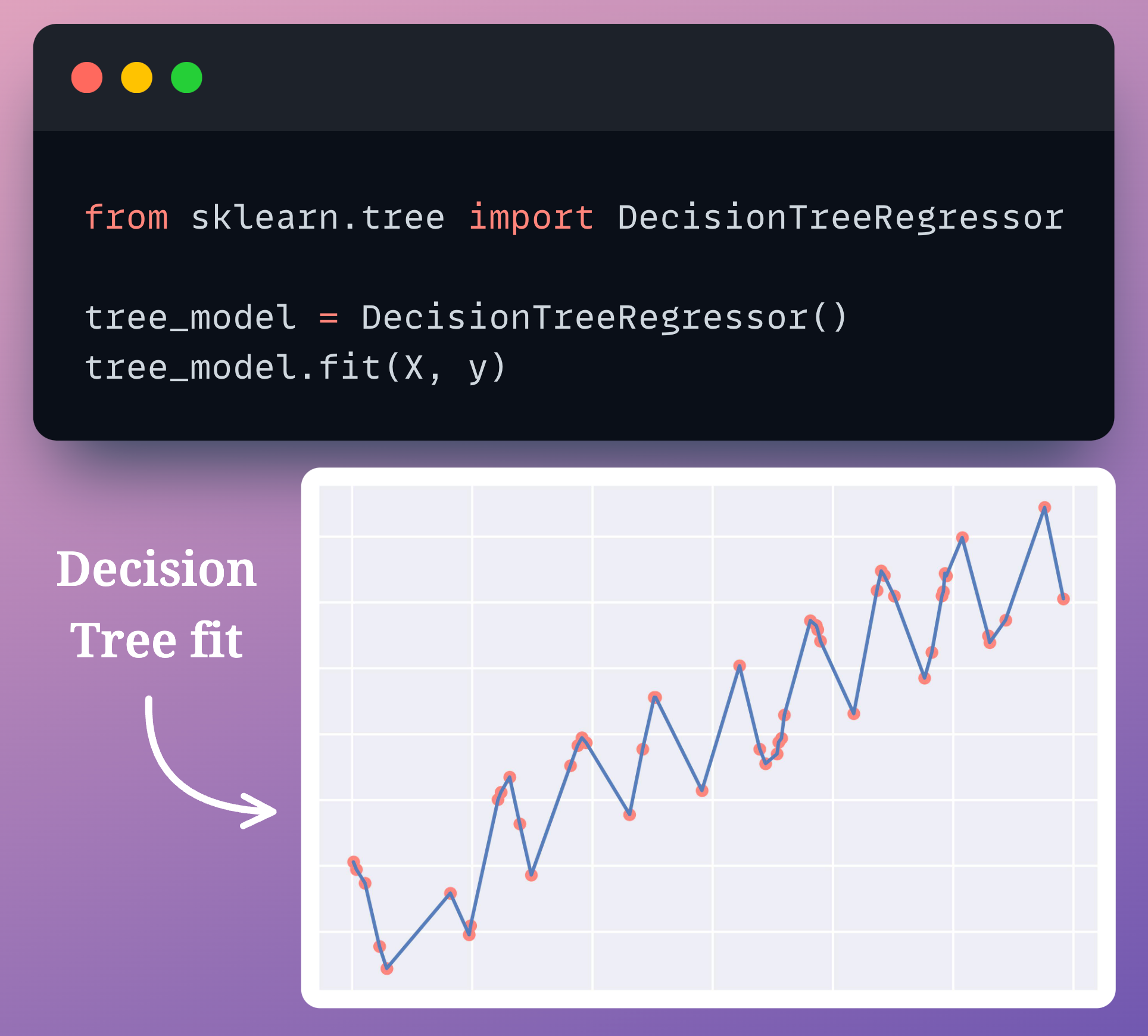
However, this is NEVER the case with a decision tree model.

In fact, overfitting any dataset with a decision tree demands no effort from the engineer.

In other words, we can simply run dtree_model.fit(X, y) to overfit any dataset, regression or classification.

This happens because a standard decision tree always continues to add new levels to its tree until all leaf nodes are pure.

As a result, it always $100\%$ overfits the dataset by default, as shown below:

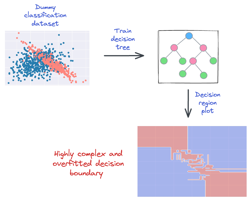
The same problem is observed in classification datasets as well.

For instance, consider the following dummy binary classification dataset.

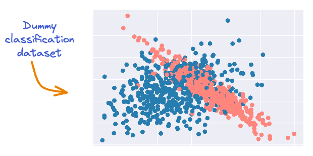
It’s clear that there is some serious overlap between the two classes.

Yet, a decision tree does not care about that.

The model will still meticulously create its decision boundary such that it classifies the dataset with 100% accuracy.

This is depicted below:

It is important to address this problem.

Remedies to Prevent Overfitting

Of course, there are many ways to prevent this, such as pruning and ensembling.

Pruning

Pruning is commonly used in tree-based models, where it involves removing branches (or nodes) to simplify the model.

For instance, we can intentionally restrict the decision tree from growing after a certain depth. In sklearn’s implementation, we can do this by specifying the max_depth parameter.

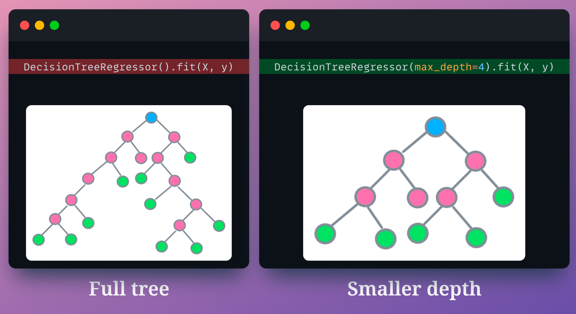
Pruning is also possible by specifying the minimum number of samples required to split an internal node.

Another pruning technique is called the cost-complexity-pruning (CCP).

CCP considers a combination of two factors for pruning a decision tree:

• Cost (C): Number of misclassifications
• Complexity (C): Number of nodes

Of course, dropping nodes will result in a drop in the model’s accuracy.

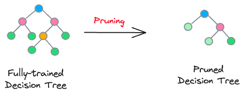
Thus, in the case of decision trees, the core idea is to iteratively drop sub-trees, which, after removal, leads to:

• a minimal increase in classification cost
• a maximum reduction of complexity (or nodes)

This is depicted below:

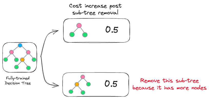
In the image above, both sub-trees result in the same increase in cost. However, it makes more sense to remove the sub-tree with more nodes to reduce computational complexity.

In sklearn, we can control cost-complexity-pruning using the ccp_alpha  parameter:

• large value of ccp_alpha → results in underfitting
• small value of ccp_alpha → results in overfitting

The objective is to determine the optimal value of ccp_alpha, which gives a better model.

The effectiveness of cost-complexity-pruning is evident from the image below:

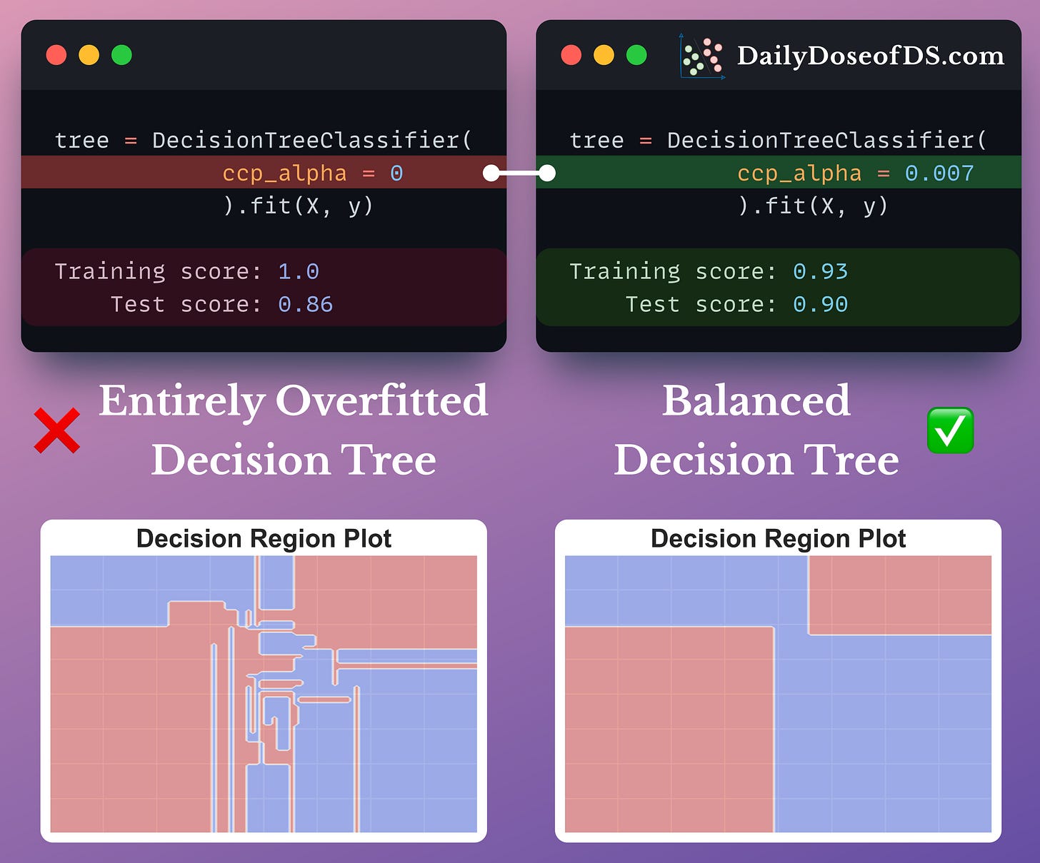
• Training the decision tree without any cost-complexity-pruning results in a complex decision region plot, and the model exhibits 100% accuracy.
• However, by tuning the ccp_alpha parameter, we prevented overfitting while improving the test set accuracy.

Ensemble learning

Another widely used technique to prevent overfitting is ensemble learning.

In a gist, an ensemble combines multiple models to build a more powerful model.

Whenever I wish to intuitively illustrate their immense power, I use the following image:

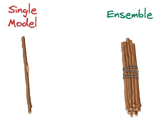
They are fundamentally built on the idea that by aggregating the predictions of multiple models, the weaknesses of individual models can be mitigated. Combining models is expected to provide better overall performance.

Ensembles are primarily built using two different strategies:

1. Bagging
2. Boosting

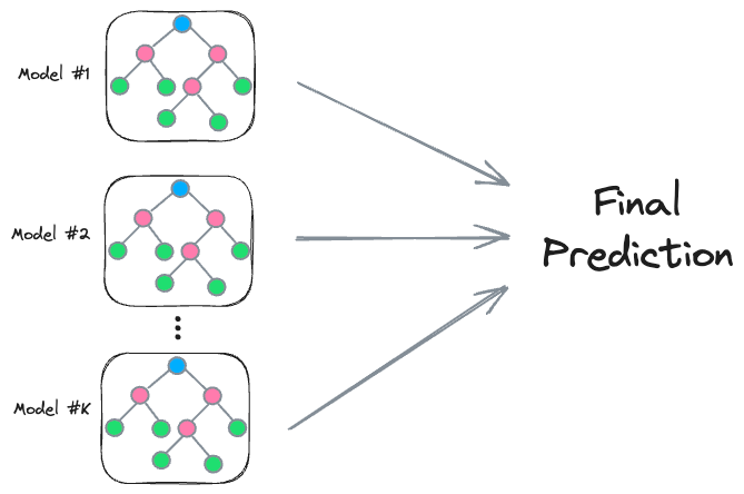
1) Bagging

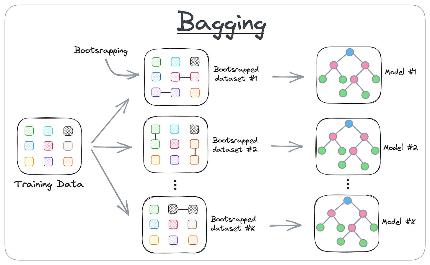
Here’s how it works:

• Bagging creates different subsets of data with replacement (this is called bootstrapping).
• Next, we train one model per subset.
• Finally, we aggregate all predictions to get the final prediction.

Some common models that leverage Bagging are:

• Random Forests
• Extra Trees

2) Boosting

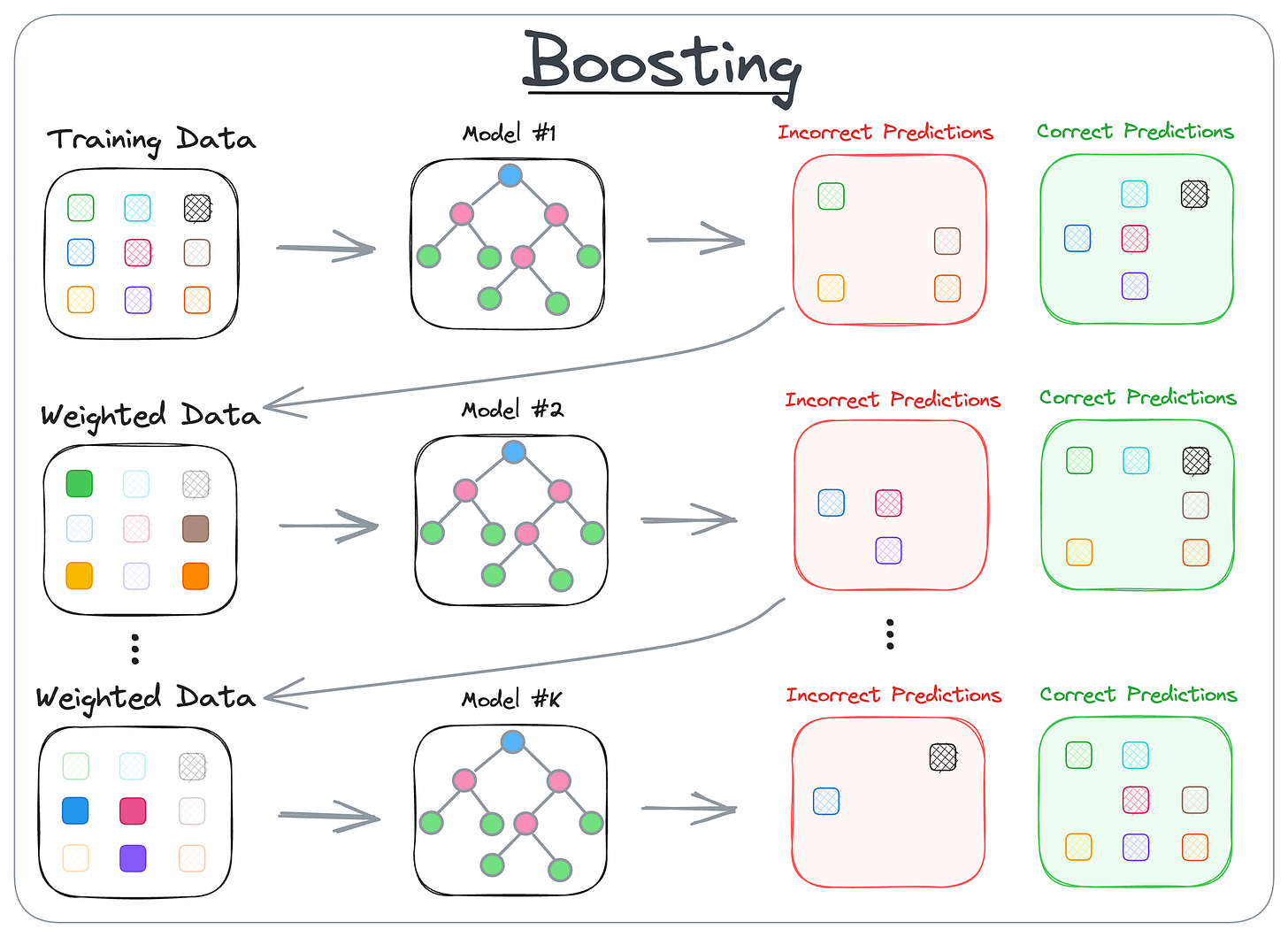
Here’s how it works:

• Boosting is an iterative training process.
• The subsequent model puts more focus on misclassified samples from the previous model
• The final prediction is a weighted combination of all predictions

Some common models that leverage Boosting are:

• XGBoost,
• AdaBoost, etc.

Overall, ensemble models significantly boost the predictive performance compared to using a single model. They tend to be more robust, generalize better to unseen data, and are less prone to overfitting.

As mentioned above, the focus of this article is specifically Bagging.

In my experience, there are plenty of resources that neatly describe:

• How Bagging algorithmically works in random forests.
• Experimental demo on how Bagging reduces the overall variance (or overfitting).

For instance, we can indeed verify variance reduction ourselves experimentally.

The following diagram shows the decision region plot obtained from a decision tree and random forest model:

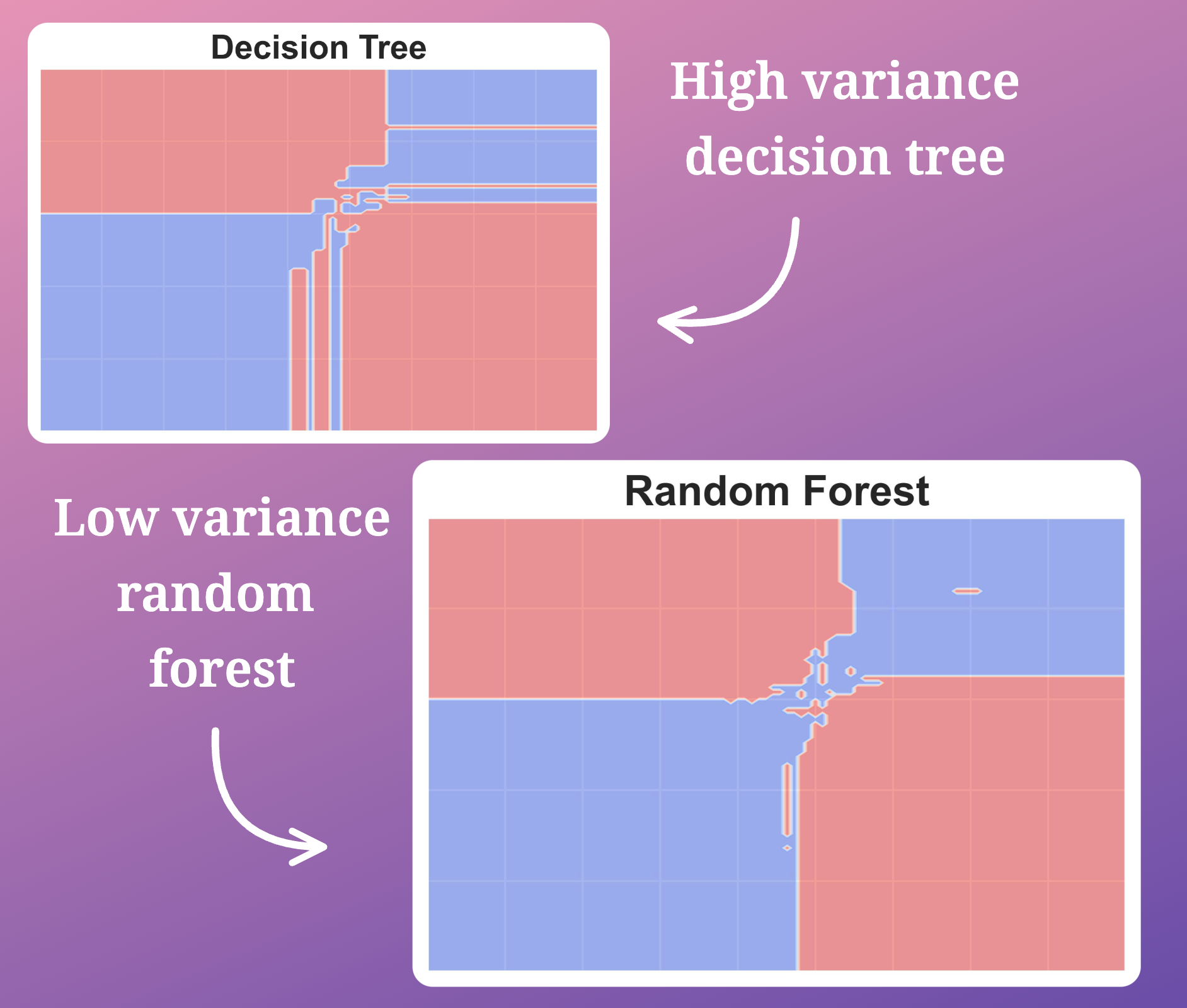
It’s pretty clear that a random forest does not exhibit as high variance (overfitting) as the decision tree model does.

Typically, these resources explain the idea of Bagging as follows:

Instead of training one decision tree, train plenty of them, each on a different subsets of the dataset generated with replacement. Once trained, average the predictions of all individual decision tree models to obtain the final prediction. This results in reducing the overall variance and increases the model’s generalization.

However, these resources often struggle to provide an intuition on:

1. Why Bagging is so effective.
2. Why do we sample rows from the training dataset with replacement.
3. The mathematical demonstration that verifies variance reduction.

Thus, in this article, let me address all of these above questions and provide you with a clear and intuitive reasoning on:

• Why bagging makes the random forest algorithm so effective at variance reduction.
• Why does bagging involves sampling with replacement?
• How do we prove variance reduction mathematically?

Towards the end, we shall also build an intuition towards the Extra trees algorithm and how it further contributes towards the variance reduction step.

Once we understand the objective bagging tries to solve, we shall also formulate new strategies to build our own bagging algorithms.

Let’s begin!

Motivation for Bagging

As shown in an earlier diagram, the core idea in a random forest model is to train multiple decision tree models, each on a different sample of the training dataset.

During inference, we take the average of all predictions to get the final prediction:

And as we saw earlier, training multiple decision trees reduces the model's overall variance.

But why?

Let’s dive into the mathematics that will explain this.