Implementing KANs From Scratch Using PyTorch

👉

Introduction

In last week's article, we understood the underlying details of Kolmogorov Arnold Networks (KAN) and how they work.

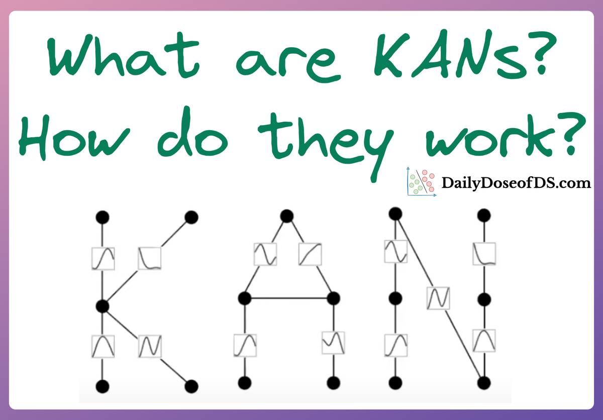
Towards the end of the article, we decided to do another article on KANs, in which we shall implement KANs using PyTorch.

Why?

I find this important because we all know how to build and train a neural network with regular weight matrices.

However, KANs are based on a different idea. The matrices KANs possess in a layer do not contain weights but functions, which are applied to the input of that layer.

Thus, by implementing KANs, we can learn how a network that does not contain the traditional weight matrices but rather univariate functions can be trained.

Let's begin!

Recap

As discussed in that article, KANs challenge traditional neural network design and offer a new paradigm to design and train them.

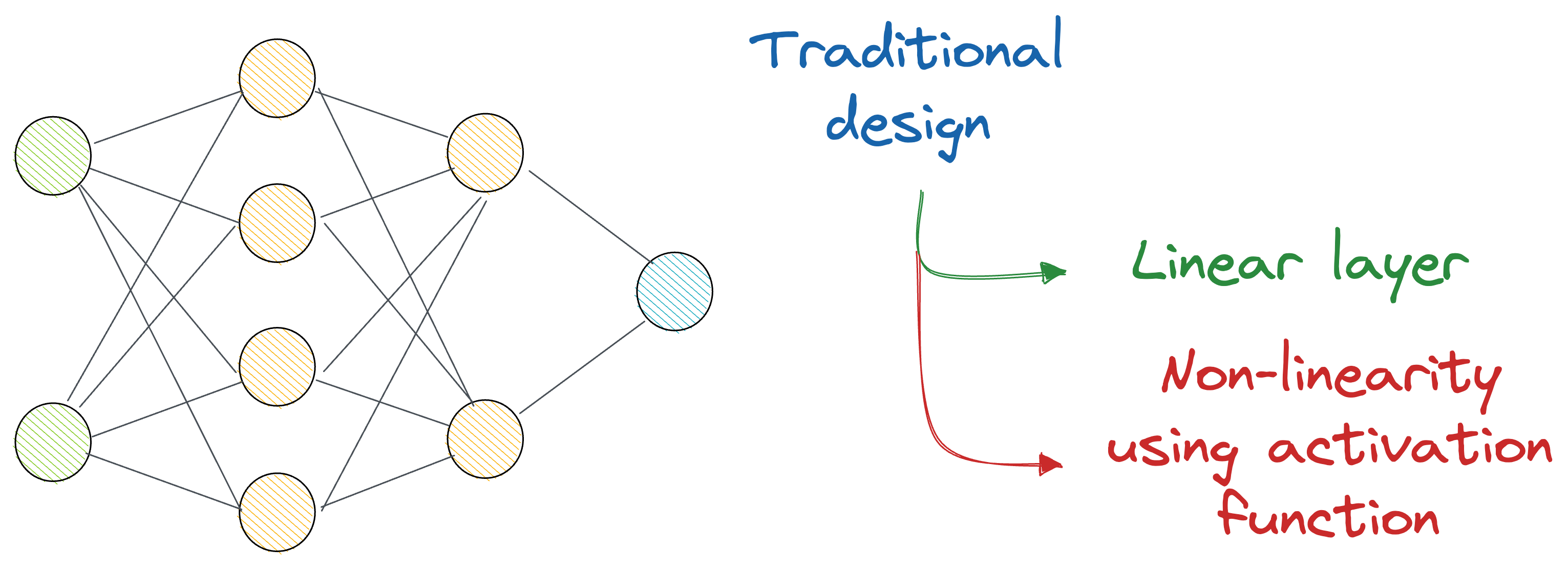
In a gist, the idea is that instead of just stacking many layers on top of each other (which are always linear transformations, and we deliberately introduce non-linearity with activation functions), KANs recommend an alternative approach.

The authors used complex learnable functions (called B-Splines) that help us directly represent non-linear input transformations with relatively fewer parameters than a traditional neural network.

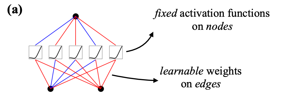
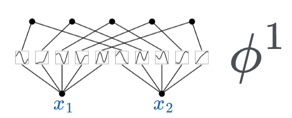
In the above image, if you notice closely:

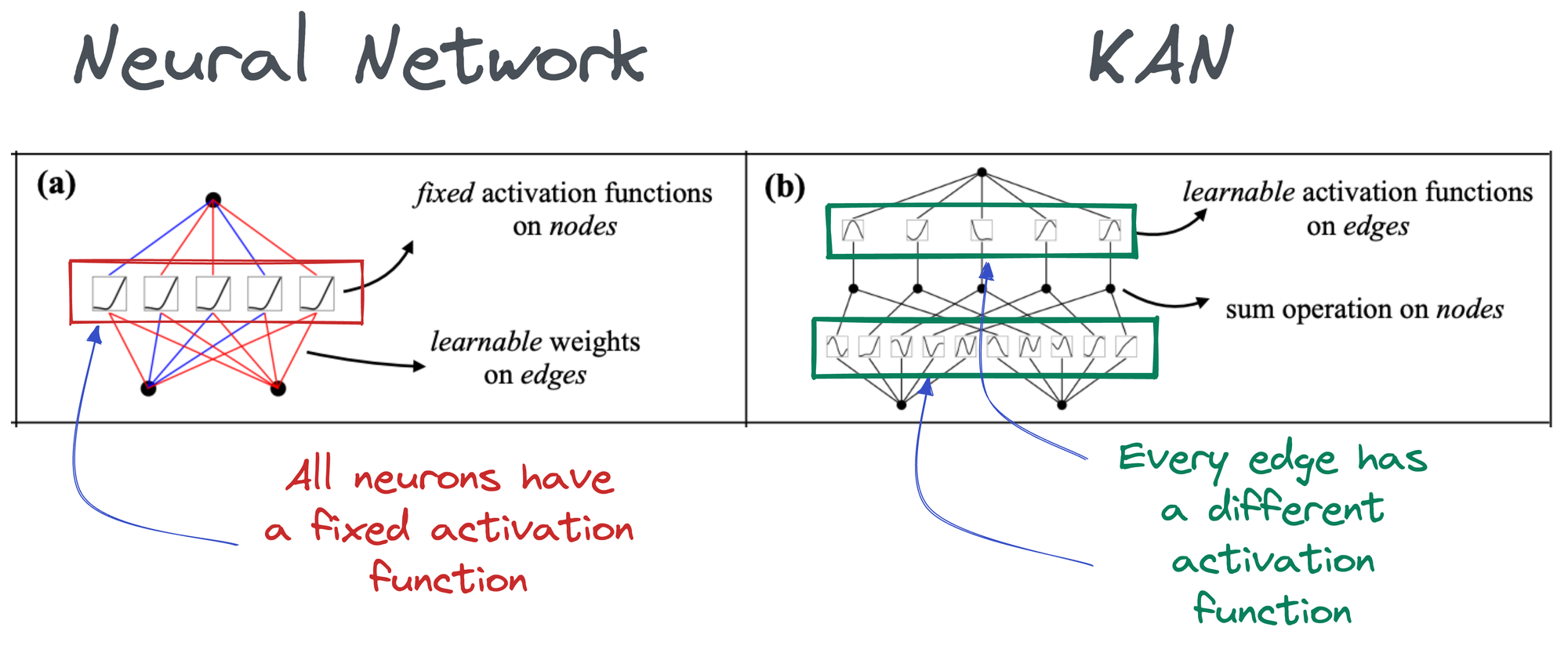
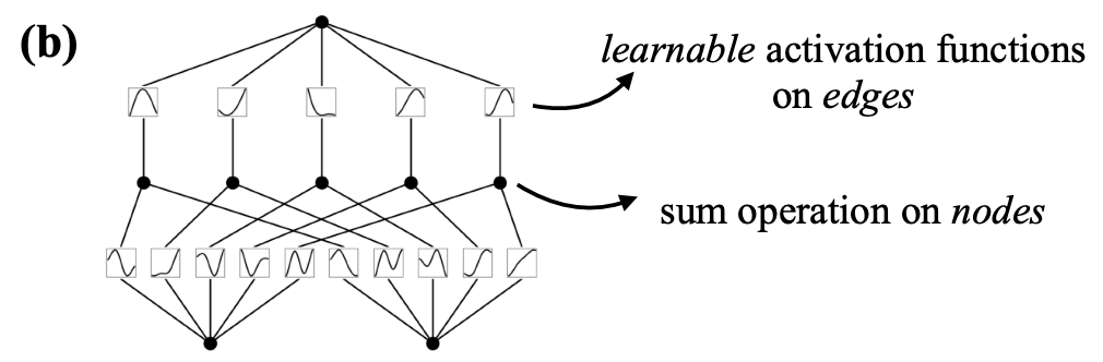
In a neural network, activation functions are fixed across the entire network, and they exist on each node (shown below).

In KAN, however, activation functions exist on edges (which correspond to the weights of a traditional neural network), and every edge has a different activation function.

Thus, it must be obvious to expect that KAN is much more accurate and interpretable with fewer parameters.

They are based on the Kolmogorov-Arnold Representation Theorem, which asserts that any multivariate continuous function can be represented as the composition of a finite number of continuous functions of a single variable.

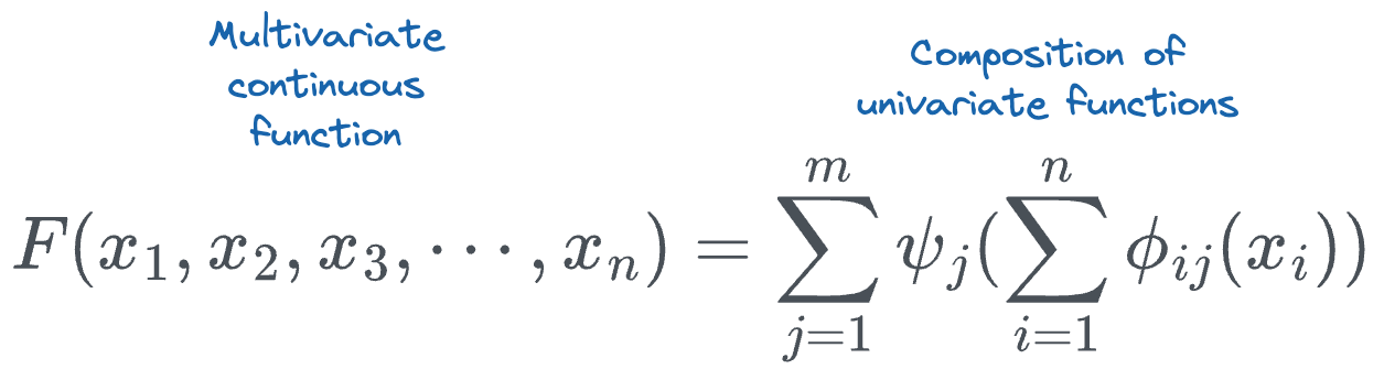
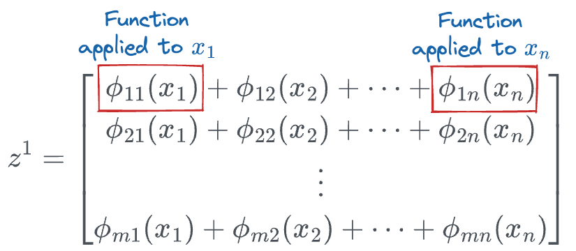
If we expand the sum terms, we get the following:

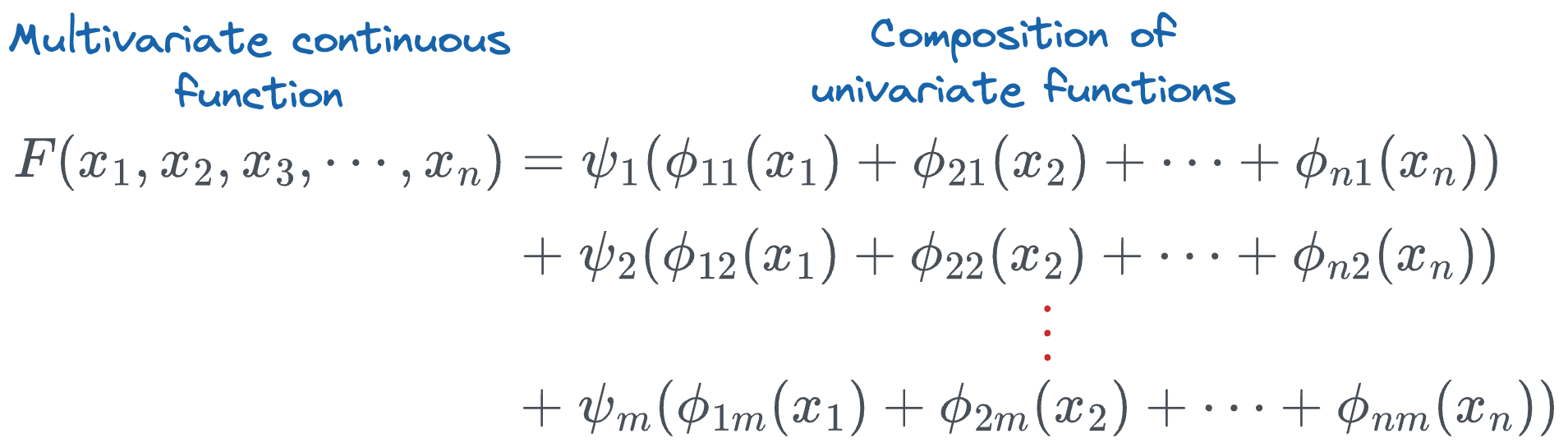
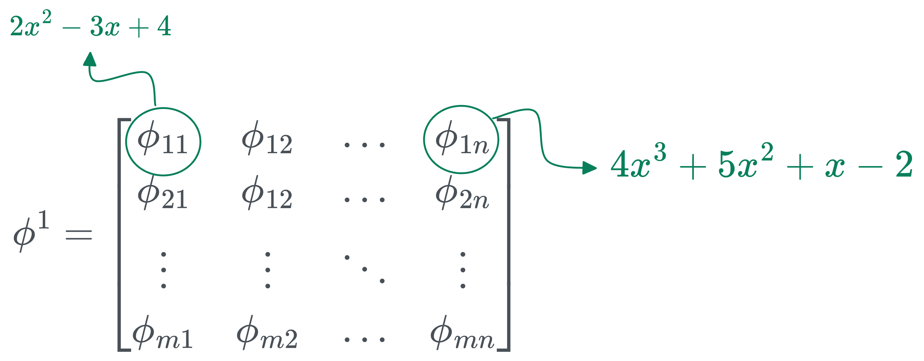
To put it all together, all we are doing in a single KAN layer is taking the input $(x_1, x_2, \cdots, x_n)$ and applying a transformation $\phi$ to it.

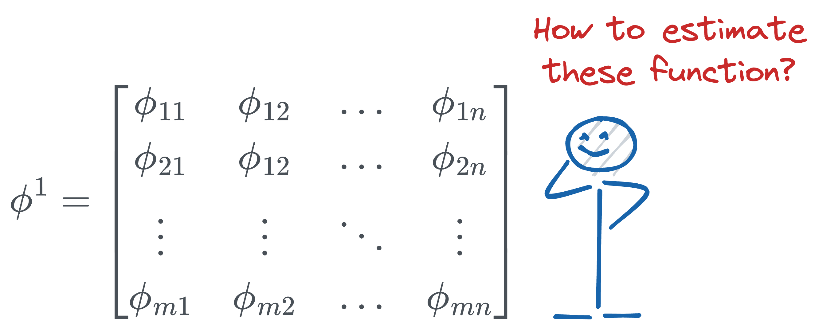
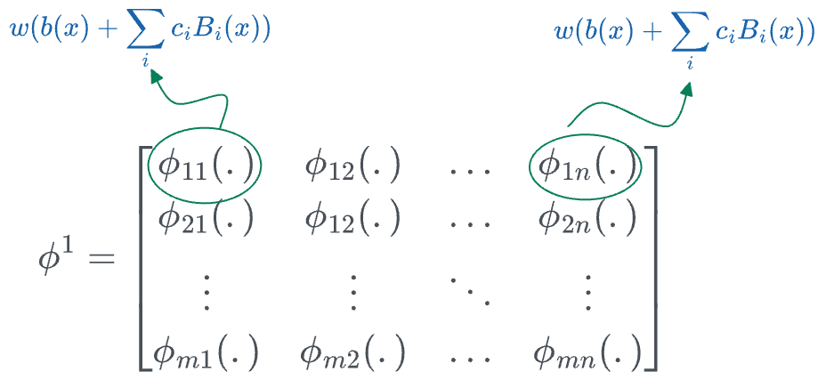
$\phi^1$ denotes the transformation in the first layer

Thus, the transformation matrix $\phi^1$ (corresponding to the first layer) can be represented as follows:

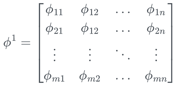
In the above matrix:

$n$ denotes the number of inputs.
$m$ denotes the number of output nodes in that layer.
[IMPORTANT] The individual entries are not numbers, they are univariate functions. For instance:
- $\phi_{11}$ could be $2x^2 - 3x + 4$.
- $\phi_{12}$ could be $4x^3 + 5x^2 + x - 2$.
- and so on...

So to generate a transformation, all we have to do is take the input vector and pass it through the corresponding functions in the above transformation matrix:

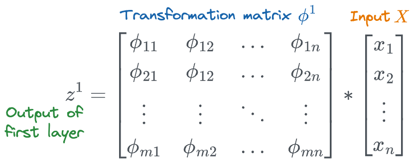
This will result in the following vector:

The above is the output of the first layer, which is then passed through the next layer for another function transformation.

Thus, the entire KAN network can be condensed into one formula as follows:

Where:

$x$ denotes the input vector
$\phi^k$ denotes the function transformation matrix of layer $k$.
$KAN(x)$ is the output of the KAN network.

In the case of KANs, the matrices $\phi^k$ themselves are non-linear transformation matrices, and each univariate function can be quite different.

But how do we estimate the univariate functions in each of the transformation matrices?

As discussed in the KANs introductory article, we do this using B-splines.

Recall that whenever we create B-splines, we already have our control points $(P_1, P_2, \dots, P_n)$, and the underlying basis functions based on the degree $k$.

And by varying the position of the control points, we tend to get different curves, as depicted in the video below:

0:00

/0:12

So here's the core idea of KANs:

Let's make the positions of control points learnable in the activation function so that the model is free to learn any arbitrary shape activation function that fits the data best.

That's it.

By adjusting the positions of the control points during training, the KAN model can dynamically shape the activation functions that best fit the data.

Start with the initial positions for the control points, just like we do with weights.
During the training process, update the positions of these control points through backpropagation, similar to how weights in a neural network are updated.
Use an optimization algorithm (e.g., gradient descent) to adjust the control points so that the model can minimize the loss function.

Mathematically speaking, in KANs, every activation function $\phi(x)$ is defined as follows:

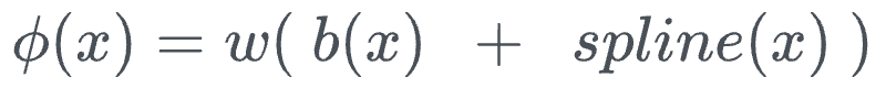
Within this:

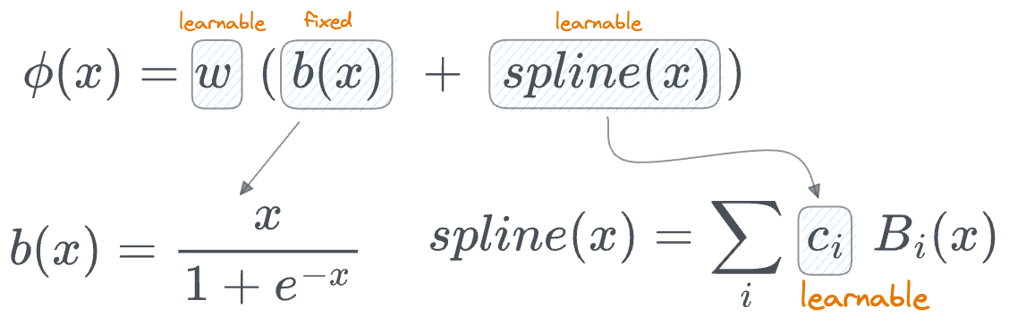
The computation involves a basis function $b(x)$ (similar to residual connections).
$spline(x)$ is learnable, specifically the parameters $c_i$, which denotes the position of the control points.
There's another parameter $w$. The authors say that, in principle, $w$ is redundant since it can be absorbed into $b(x)$ and $spline(x)$. Yet, they still included this $w$ factor to better control the overall magnitude of the activation function.

Once this has been defined, the network can be trained just like any other neural network.

More specifically: