Formulating the Principal Component Analysis (PCA) Algorithm From Scratch
Approaching PCA as an optimization problem.
Dimensionality reduction is crucial to gain insight into the underlying structure of high-dimensional datasets.
One technique that typically stands out in this respect is the Principal Component Analysis (PCA).
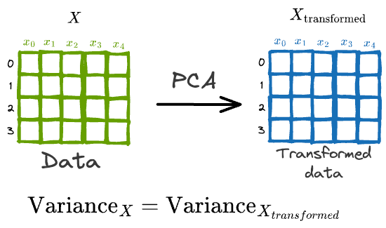
In a gist, the core objective of PCA is to transform the data $X$ into another space such that new features are uncorrelated and preserve the variance of the original data.
While PCA is widely popular, I have noticed that most folks struggle to design its true end-to-end formulation from scratch.
Many try to explain PCA by relating it to the idea of eigenvectors and eigenvalues, which is true — PCA does perform transformations using eigenvectors and eigenvalues.
But why?
There are two questions to ask here:
- How can we be sure that the data projections that involve eigenvectors and eigenvalues in PCA is the most obvious solution to proceed with?
- How can we be sure that the above transformation does preserve the data variance?
In other words, where did this whole notion of eigenvectors and eigenvalues originate from in PCA?
I have always believed that it is not only important to be aware of techniques, but it is also crucial to know how these techniques are formulated end-to-end.
And the best way to truly understand any algorithm or methodology is by manually building it from scratch.
It is like replicating the exact thought process when someone first designed the algorithm by approaching the problem logically, with only mathematical tools.
Thus, in this dimensionality-reduction article series, we’ll dive deep into one of the most common techniques: Principal Component Analysis (PCA)
We’ll look at:
- The intuition and the motivation behind dimensionality reduction.
- What are vector projections and how do they alter the mean and variance of the data?
- What is the optimization step of PCA?
- What are Lagrange Multipliers and how are they used in PCA optimization?
- What is the final solution obtained by PCA?
- How to determine the number of components in PCA?
- Why should we be careful when using PCA for visualization?
- What are the advantages and disadvantages of PCA?
- Takeaways.
Let’s begin!
Principal Component Analysis (PCA)
Motivation for dimensionality reduction
Imagine someone gave you the following weight and height information about a few individuals:
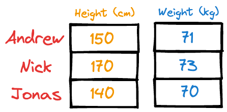
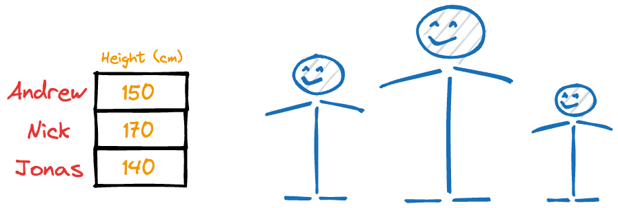
It is easy to guess that the height column has more variation than weight.
Thus, even if you were to discard the weight column, chances are you could still identify these individuals solely based on their heights.
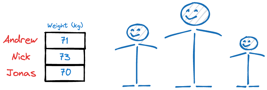
However, if you were to discard the height column, you would likely struggle to identify them.
Why?
Because their heights have more variations than their weights, and it’s clear from this example that, typically, if the data has more variation, it holds more information (this might not always be true, though, and we’ll learn more about this later).
That’s the essence of many dimensionality reduction techniques.
Simply put, we reduce dimensions by eliminating useless (or least useful) features.
Based on this explanation, one plausible and intuitive way might be to measure column-wise variance and eliminate top $k$ features with the least variance.
This is depicted below:
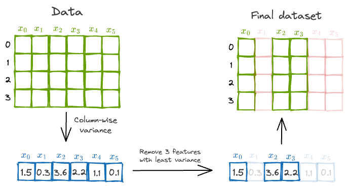
However, there’s a problem with this approach.
Almost all datasets have correlated features. Thus, in the case of high correlation, this puts a challenge on which feature we should eliminate or retain in the final dataset.
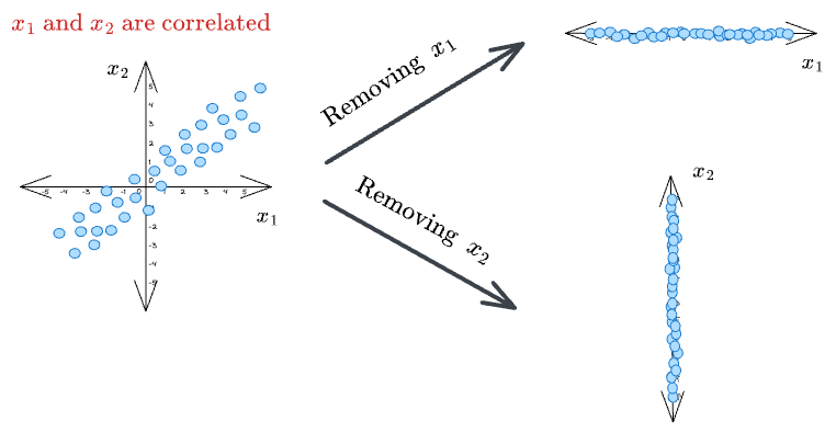
Removing one feature that is highly correlated with another may lead to an incoherent dataset, as both features can be equally important. As a result, it may lead to misleading conclusions.
Thus, the above approach of eliminating features based on feature variance is only ideal if the features we begin with are entirely uncorrelated.
So, can we do something to make the features in our original dataset uncorrelated?
Can we apply any transformation that does this?
Of course we can!
For instance, consider the above dummy dataset again where $x_1$ and $x_2$ were correlated:
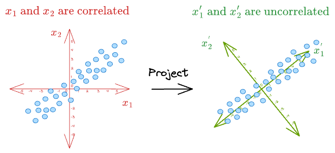
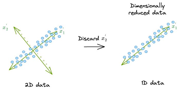
As shown above, if we can represent the data in a new coordinate system $(x_1^{'}, x_2^{'})$, it is easy to see that there is almost no correlation between the new features.
What's more, the data varies mostly along the dimension $(x_1^{'})$.
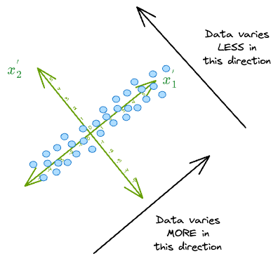
As a result, in this new coordinate system, we can safely discard the dimension along which the original data has the least variance, i.e., $(x_2^{'})$.
Think of it this way. If we were to discard the dimension $(x_1^{'})$, we would get the following low-dimensional representation of the data:
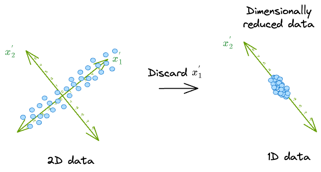
It makes much more sense to discard $(x_2^{'})$ because the data varies less along that dimension.
So overall, these are the steps we need to follow:
Step #1) Develop a new coordinate system for our data such that the new features are uncorrelated.
Step #2) Find the variance along each of the new uncorrelated features.
Step #3) Discard the features with the least variance to get the final “dimensionally-reduced dataset.”
Here, it is easy to guess that steps $2$ and $3$ aren’t that big of a challenge. Once we have obtained the new uncorrelated features, the only objective is to find their variance and discard the features with the least variances.
Thus, the primary objective is to develop the new coordinate system, $(x_1^{'}, x_2^{'})$ in the above illustration.
In other words, we want to project the data to a low-dimensional space to preserve as much of the original variance as possible while effectively reducing the dimensions.
As we’ll look shortly, this becomes more like an optimization problem.
So, how do we figure out the best projection for our data?
Vector projection, projection mean, and projection variance
As the name suggests, vector projection is about finding the component of one vector that lies in the direction of another vector.
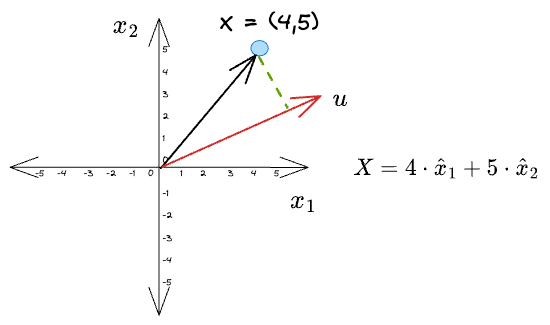
For instance, consider a toy example:
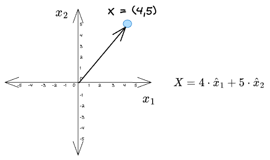
Given a vector $X = (4, 5)$, its projections along the coordinate axes $\hat x_1$ and $\hat x_2$ are:
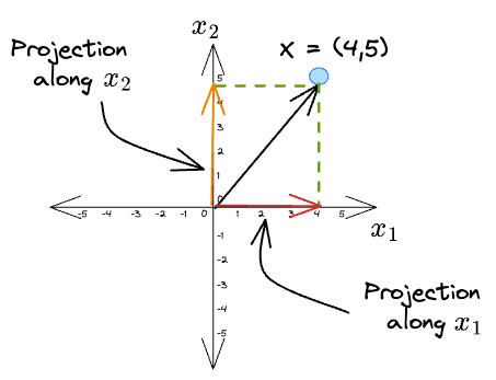
What we did was we projected the original vector along the direction of some other vector.
A little complicated version of this could be to project it along a vector that is different from the coordinate vectors, $u$ in the following figure:
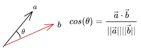
For simplicity, let’s consider the vector $u$ to be a unit vector — one which has a unit length.
By the notion of cosine similarity, we know that the cosine of the angle between two vectors is given by:
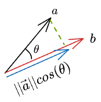
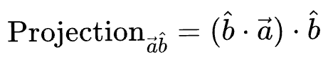
Thus, we can write the length of the projection of $\vec{a}$ on $\vec{b}$ as:
Now, we know the magnitude of the projection. Next, we can do a scaler vector multiplication of this magnitude with the unit vector in the desired direction ($\hat b$) to get the projection vector:
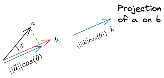
Substituting the value of $cos(\theta)$, and simplifying we get the final projection as:
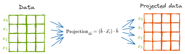
Until now, we considered just one data point for projection. But our dataset will indeed have many more data points.
The above projection formula will still hold.
In other words, we can individually project each of the vectors as depicted below:
However, the projection will alter the mean and variance of the individual features.
But it’s simple to figure out the new mean and variance after the projection.
Essentially, all data points are vectors in some high-dimensional space. Thus, the mean of the individual features will also be a vector in that same space $(\hat \mu)$.
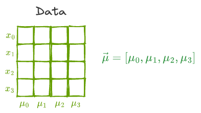
As a result, it makes intuitive sense that the transformation to the individual data points will equally affect the mean vector as well.
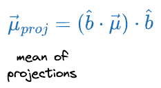
With this in mind, we can get the projected mean vector as follows:
Similarly, we can also determine the variance of the individual features after projection as follows:
So, to summarize, if we are given some data points X as follows:
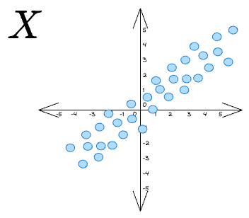
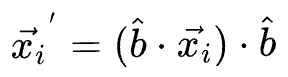
If we want to project these vectors along some unit vector $\hat b$:
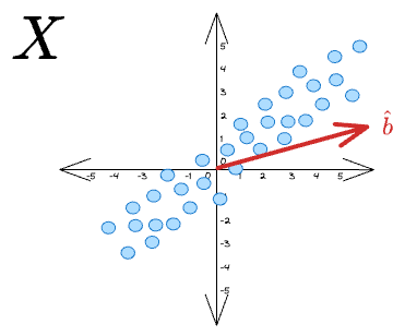
...then the projection for a specific data point $x_i$ is given by:
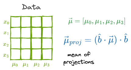
If the individual features had a mean vector $\vec{\mu}$, then the mean of the projections is given by:
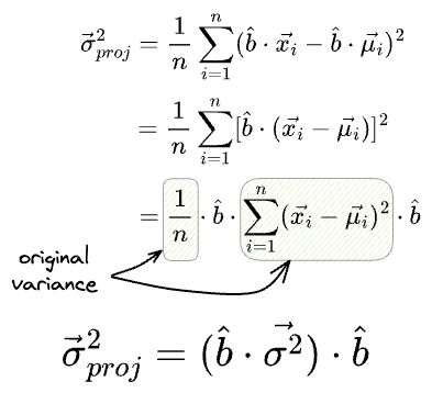
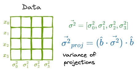
What’s more, if the individual features had a variance vector $\vec{\sigma^2}$, then the variance of the projections is given by:
Finally, the idea of finding the variance of the projection can be extended to the covariance matrix of the projection as well.
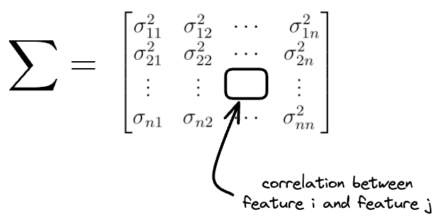
In simple terms, while variance $\vec{\sigma^2}$ above denoted the individual feature variances, the covariance matrix holds the information about how two features vary together.
Say $\sum$ denotes the covariance matrix for the original features:
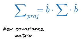
Then the covariance matrix of the projections $\sum_{proj}$ can be written as:
PCA optimization step
With this, we are set to proceed with formulating PCA as an optimization problem.