Build and Deploy Agents to Production

Hands-on

​Build and deploy Agents to production​

We have been building AI Agents in production for over an year.

If you want to learn too, we have put together a simple hands-on tutorial for you.

We build and deploy a Coding Agent that can scrape docs, write production-ready code, solve issues, and raise PRs, directly from Slack.

Tech Stack:

• Claude Code for code generation
• ​xpander​ as the Agent backend
• ​Firecrawl​ for web scraping

For context...

​xpander​ is a plug-and-play Backend for agents that manages scale, memory, tools, multi-user states, events, guardrails, and more.

Once we deploy an Agent, it also provides various triggering options like MCP, Webhook, SDK, Chat, etc.

Moreover, you can also integrate any Agent directly into Slack with no manual OAuth setups, no code, and no infra headaches.

One good thing is that this Slack Agent natively supports messages with audio, images, PDFs, etc.

Note: If you want to learn how to build Agentic systems, we have published 6 parts so far in our Agents crash course (with implementation):

• ​Part 1 → Why Agents? Creating Agents, Tasks, Tools, etc.​
• ​Part 2 → Modular agents, custom tools, structured outputs, etc.​
• ​Part 3 → Agentic Flows.​
• ​Part 4 → Hands-on deep dive on building 2 agentic Flows systems.​
• Part 5​ and ​Part 6​ → Advanced techniques to build robust Agents.

machine learning

​The intuition behind using ‘Variance’ in PCA​​

PCA is built on the idea of variance preservation.

The more variance we retain when reducing dimensions, the less information is lost.

Here’s an intuitive explanation of this.

Imagine you have the following data about three people:

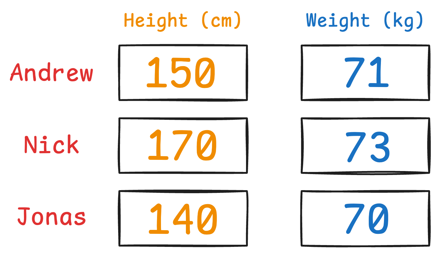
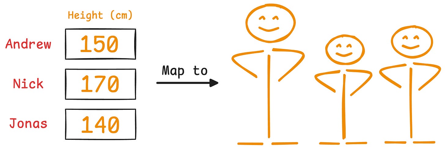
It is clear that height has more variance than weight.

Even if we discard the weight, we can still identify them solely based on height.

But if we discard the height, it’s a bit difficult to identify them now:

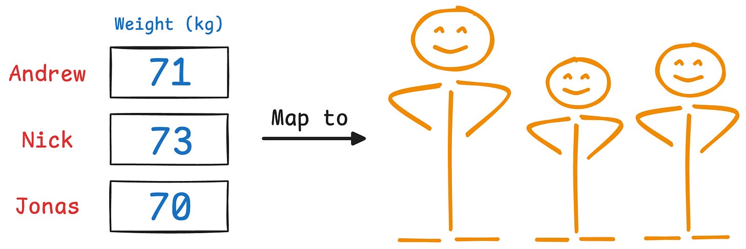
This is the premise on which PCA is built.

More specifically, during dimensionality reduction, if we retain more original data variance, we retain more information.

Of course, since it uses variance, it is influenced by outliers.

That said, in PCA, we don’t just measure column-wise variance and drop the columns with the least variance.

Instead, we transform the data to create uncorrelated features and then drop the new features based on their variance.

To dive into more mathematical details, we formulated the entire PCA algorithm from scratch here: ​Formulating PCA Algorithm From Scratch​, where we covered:

• What are vector projections, and how do they alter the mean and variance of the data?
• What is the optimization step of PCA?
• What are Lagrange Multipliers?
• How are Lagrange Multipliers used in PCA optimization?
• What is the final solution obtained by PCA?
• Proving that the new features are indeed uncorrelated.
• How to determine the number of components in PCA?
• What are the advantages and disadvantages of PCA?
• Key takeaways.

And in the follow-up part to PCA, we formulated tSNE from scratch, an algorithm specifically designed to visualize high-dimensional datasets.

We also implemented tSNE with all its backpropagation steps from scratch using NumPy.

Read here: ​Formulating and Implementing the t-SNE Algorithm From Scratch.​​

machine learning

​A point of caution when using one-hot encoding​

One-hot encoding introduces a problem in the dataset.

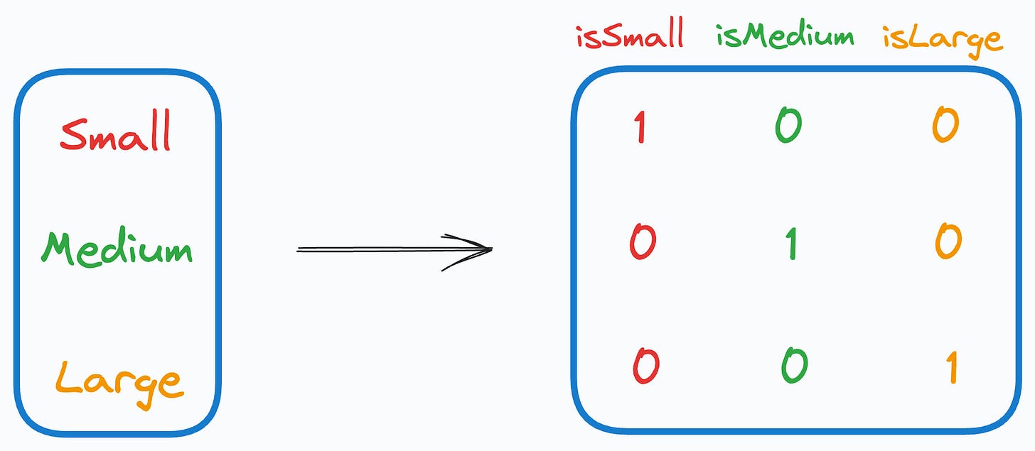
More specifically, when we use it, we unknowingly introduce perfect multicollinearity.

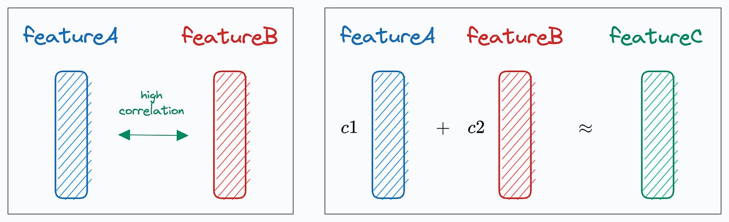
Multicollinearity arises when two (or more) features are highly correlated OR two (or more) features can predict another feature:

In our case, as the sum of one-hot encoded features is always 1, it leads to perfect multicollinearity, and it can be problematic for models that don’t perform well under such conditions.

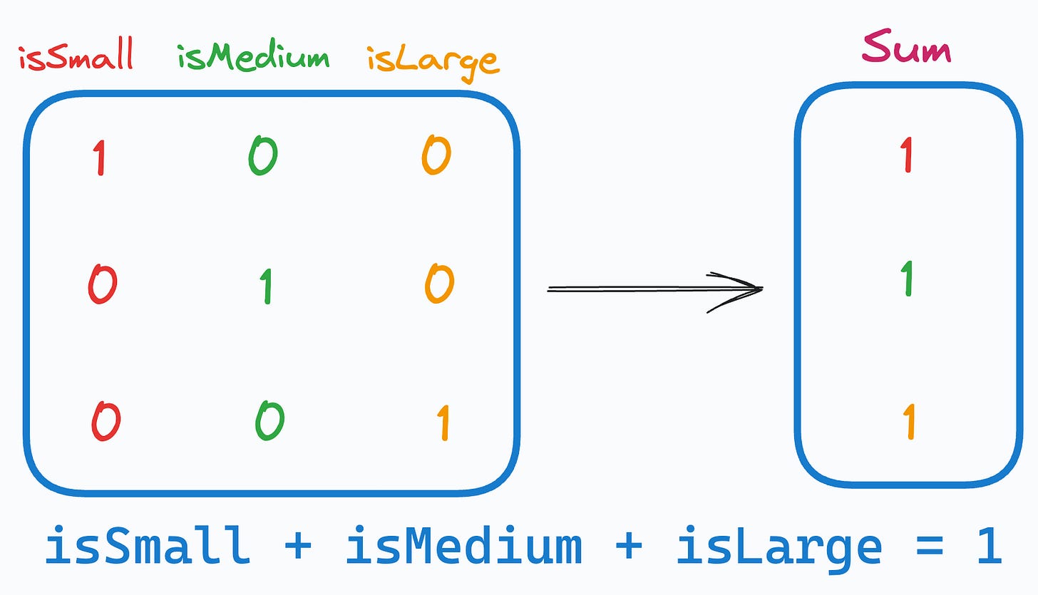
This problem is often called the Dummy Variable Trap.

Talking specifically about linear regression, for instance, it is bad because:

• In some way, our data has a redundant feature.
• Regression coefficients aren’t reliable in the presence of multicollinearity, etc.

That said, the solution is pretty simple.

Drop any arbitrary feature from the one-hot encoded features.

This instantly mitigates multicollinearity and breaks the linear relationship that existed before, as depicted below:

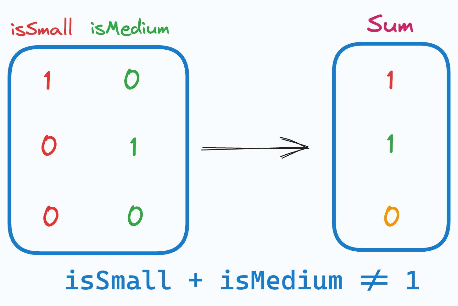
The above way of categorical data encoding is also known as dummy encoding, and it helps us eliminate the perfect multicollinearity introduced by one-hot encoding.

​We covered 8 fatal (yet non-obvious) pitfalls (with measures) in DS here →