Model Compression: A Critical Step Towards Efficient Machine Learning
Four critical ways to reduce model footprint and inference time.
Motivation
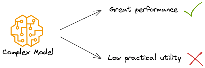
Training machine learning (ML) models are frequently driven by a relentless pursuit of achieving higher and higher accuracies.
Many create increasingly complex deep learning models, which, without a doubt, do incredibly well “performance-wise.”
However, the complexity severely impacts their real-world utility.
For years, the primary objective in model development has been to achieve the best performance metrics.
However, it is important to note that when it comes to deploying these models in production (or user-facing) systems, the focus shifts from raw accuracy to considerations such as efficiency, speed, and resource consumption.
Thus, typically, when we deploy any model to production, the specific model that gets shipped to production is NOT solely determined based on performance.
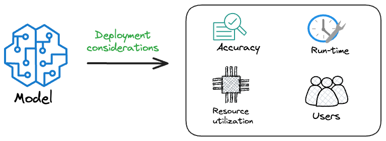
Instead, we must consider several operational metrics that are not ML-related.
What are they? Let’s understand!
Typical operational metrics
When a model is deployed into production, certain requirements must be met.
Typically, these “requirements” are not considered during the prototyping phase of the model.
For instance, it is fair to assume that a user-facing model may have to handle plenty of requests from a product/service the model is integrated with.
And, of course, we can never ask users to wait for, say, a minute for the model to run and generate predictions.
Thus, along with “model performance,” we would want to optimize for several other operational metrics:
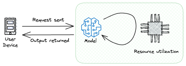
#1) Inference latency
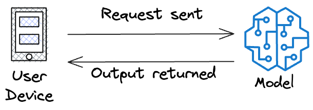
It’s the time it takes for a model to process a single input and generate a prediction.
It measures the delay between sending a request to the model and receiving the response.
Striving for a low inference latency is crucial for all real-time or interactive applications, as users expect a quick response.
High latency, as you may have guessed, will lead to a poor user experience and will not be suitable for many applications like:
- Chatbots
- Real-time speech-to-text transcription
- Gaming, and many more.
#2) Throughput
Throughput is the number of inference requests a model can handle in a given time period.
It estimates the model’s ability to process multiple requests simultaneously.
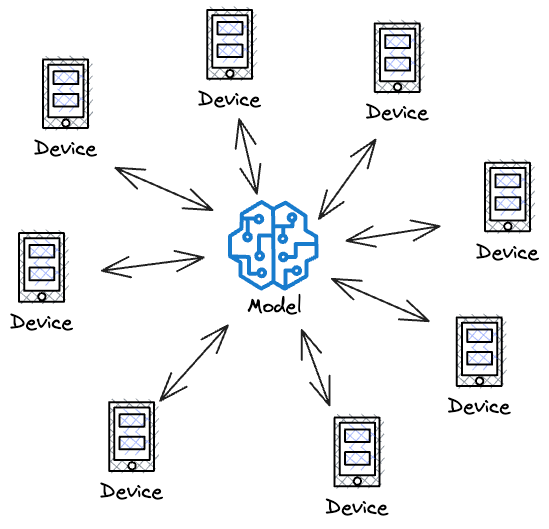
Yet again, as you may have guessed, high throughput is essential for applications with a high volume of incoming requests.
These include e-commerce websites, recommendation systems, social media platforms, etc. High throughput ensures that the model can serve many users concurrently without significant delays.
#3) Model size
This refers to the amount of memory a model occupies when loaded for inference purposes.
It quantifies the memory footprint required to store all the parameters, configurations, and related data necessary for the model to make predictions or generate real-time outputs.
The significance of model size becomes particularly apparent when deploying models in resource-constrained environments.
Many production environments, such as mobile devices, edge devices, or IoT devices, have limited memory capacity.
It is obvious to guess that in such cases, the model’s size will directly impact whether it can be deployed at all.
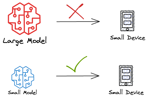
Large models may not fit within the available memory, making them impractical for these resource-constrained settings.
A real-life instance
This is a famous story.
In 2006, Netflix launched the “Netflix Prize,” a machine learning competition that encouraged ML engineers to build the best algorithm to predict user ratings for films.
The grand prize was USD $ 1,000,000 $.
After the competition concluded, Netflix awarded a $1 million prize to a developer team in 2009 for an algorithm that increased the accuracy of the company's recommendation engine by 10 percent.
That’s a lot!
Yet, Netflix never used that solution because it was overly complex.
Here’s what Netflix said:
The increase in accuracy of the winning improvements did not seem to justify the engineering effort needed to bring them into a production environment.
The complexity and resource demands of the developed model made it impractical for real-world deployment. Netflix faced several challenges:
- Scalability: The model was not easily scalable to handle the vast number of users and movies on the Netflix platform. It would have required significant computational resources to make real-time recommendations for millions of users they had.
- Maintenance: Managing and updating such a complex model in a production environment would have been a logistical nightmare. Frequent updates and changes to the model would be challenging to implement and maintain.
- Latency: The ensemble model's inference latency was far from ideal for a streaming service. Users expect near-instantaneous recommendations, but the complexity of the model made achieving low latency difficult.
You can read more about this story here: Netflix Prize story.
Consequently, Netflix never integrated the winning solution into its production recommendation system. Instead, they continued to use a simplified version of their existing algorithm, which was more practical for real-time recommendations.
This real-life instance from the Netflix Prize was a reminder that we must strive for a delicate balance between model complexity and practical utility.
While highly complex models may excel in research and competition settings, they may not be suitable for real-world deployment due to scalability, maintenance, and latency concerns.
In practice, simpler and more efficient models often are a better choice for delivering a seamless user experience in production environments.
Let me ask you this. Which of the following two models would you prefer to integrate into a user-facing product?
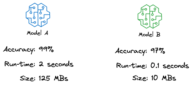
I strongly prefer Model B.
If you understand this, you resonate with the idea of keeping things simple in production.
Fortunately, there are various techniques that can help us reduce the size of the model, thereby increasing the speed of model inference.
These techniques are called Model Compression methods.
Using these techniques, you can reduce both the latency and size of the original model.
Model Compression
As the name suggests, model compression is a set of techniques used to reduce the size and computational complexity of a model while preserving or even improving its performance.

They aim to make the model smaller — that is why the name “model compression.”
Typically, it is expected that a smaller model will:
- Have a lower inference latency as smaller models can deliver quicker predictions, making them well-suited for real-time or low-latency applications.
- Be easy to scale due to their reduced computational demands.
- Have a smaller memory footprint.
In this article, we’ll look at four techniques that help us achieve this:
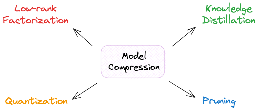
- Knowledge Distillation
- Pruning
- Low-rank Factorization
- Quantization
As we will see shortly, these techniques attempt to strike a balance between model size and accuracy, making it relatively easier to deploy models in user-facing products.
Let’s understand them one by one!
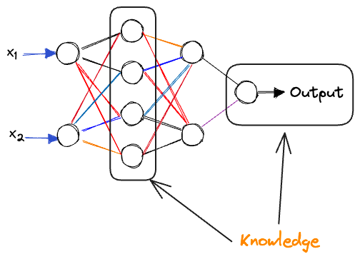
#1) Knowledge Distillation
This is one of the most common, effective, reliable, and one of my favorite techniques to reduce model size.
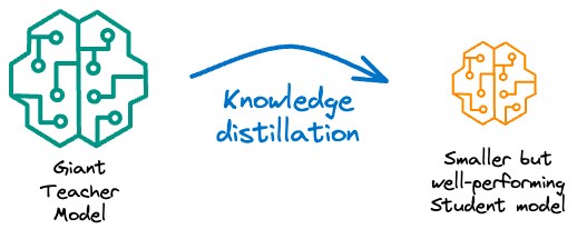
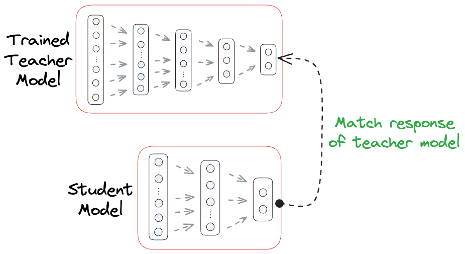
Essentially, knowledge distillation involves training a smaller, simpler model (referred to as the “student” model) to mimic the behavior of a larger, more complex model (known as the “teacher” model).
The term can be broken down as follows:
- Knowledge: Refers to the understanding, insights, or information that a machine learning model has acquired during training. This “knowledge” can be typically represented by the model’s parameters, learned patterns, and its ability to make predictions.
- Distillation: In this context, distillation means transferring or condensing knowledge from one model to another. It involves training the student model to mimic the behavior of the teacher model, effectively transferring the teacher's knowledge.
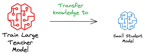
This is a two-step process:
- Train the large model as you typically would. This is called the “teacher” model.
- Train a smaller model, which is intended to mimic the behavior of the larger model. This is also called the “student” model.
The primary objective of knowledge distillation is to transfer the knowledge, or the learned insights, from the teacher to the student model.
This allows the student model to achieve comparable performance with fewer parameters and reduced computational complexity.
The technique makes intuitive sense as well.
Of course, comparing it to a real-world teacher-student scenario in an academic setting, the student model may never perform as well as the teacher model.
But with consistent training, we can create a smaller model that is almost as good as the larger one.
This goes back to the objective we discussed above
Strike a balance between model size and accuracy, such that it is relatively easier to deploy models in user-facing products.
A classic example of a model developed in this way is DistillBERT. It is a student model of BERT.
We also discussed this in the newsletter here:
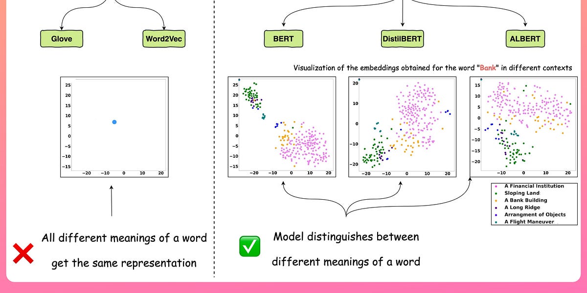
DistilBERT is approximately $40\%$ smaller than BERT, which is a massive difference in size.
Still, it retains approximately $97\%$ of the natural language understanding (NLU) capabilities of BERT.
What’s more, DistilBERT is roughly 60% faster in inference.
This is something I have personally experienced and verified in one of my research studies on Transformer models:
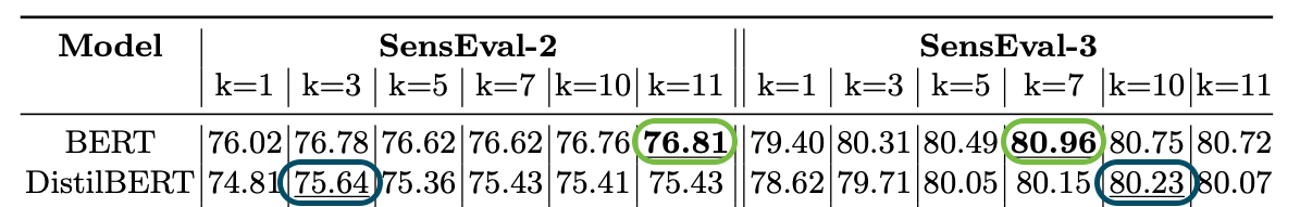
As shown above, on one of the studied datasets (SensEval-2), BERT achieved the best accuracy of $76.81$. With DistilBERT, it was $75.64$.
On another task (SensEval-3), BERT achieved the best accuracy of $80.96$. With DistilBERT, it was $80.23$.
Of course, DistilBERT isn’t as good as BERT. Yet, the performance difference is small.
Given the run-time performance benefits, it makes more sense to proceed with DistilBERT instead of BERT in a production environment.
One of the biggest downsides of knowledge distillation is that one must still train a larger teacher model first to train the student model.
However, in a resource-constrained environment, it may not be feasible to train a large teacher model.
Assuming we are not resource-constrained at least in the development environment, one of the most common techniques for Knowledge Distillation is Response-based Knowledge Distillation.
As the name suggests, in response-based knowledge distillation, the focus is on matching the output responses (predictions) of the teacher model and the student model.
Talking about a classification use case, this technique transfers the probability distributions of class predictions from the teacher to the student.
It involves training the student to produce predictions that are not only accurate but also mimic the soft predictions (probability scores) of the teacher model.
As we are trying to mimic the probability distribution of the class predictions of the teacher model, one ideal candidate for the loss function is KL divergence.
We discussed this in detail in one of the previous articles on t-SNE.
Yet, here’s a quick recap:
KL divergence
The core idea behind KL divergence is to assess how much information is lost when one distribution is used to approximate another.
Thus, the more information is lost, the more the KL divergence. As a result, the more the dissimilarity.
KL divergence between two probability distributions $P(x)$ and $Q(x)$ is calculated as follows:
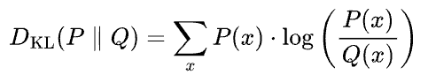
The formula for KL divergence can be read as follows:
The KL divergence $D_{KL} (P || Q) $ between two probability distributions $P$ and $Q$ is calculated by summing the above quantity over all possible outcomes $x$. Here:
- $P(x)$ represents the probability of outcome $x$ occurring according to distribution $P$.
- $Q(x)$ represents the probability of the same outcome occurring according to distribution $Q$.
It measures how much information is lost when using distribution $Q$ to approximate distribution $P$.
Imagine this. Say $P$ and $Q$ were identical. This should result in zero loss of information. Let’s verify this from the formula above.
If the probability distributions $P$ and $Q$ are identical, it means that for every $x$, $P(x) = Q(x)$. Thus,
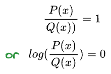
Simplifying, we get:
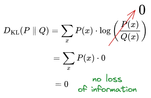
This is precisely what we intend to achieve in response-based knowledge distillation.
Simply put, we want the probability distribution of the class predictions of the student model to be identical to the probability distribution of the class predictions of the teacher model.
- First, we can train the teacher model as we typically would.
- Next, we can instruct the student model to mimic the probability distribution of the class predictions of the teacher model.
Let’s see how we can practically use response-based knowledge distillation using PyTorch.
More specifically, we shall train a slightly complex neural network on the MNIST dataset. Then, we will build a simpler neural network using the response-based knowledge distillation technique.
Step 1) Import required packages and libraries
First, we import the required packages from PyTorch:
Step 2) Load the dataset
Next, we load the MNIST dataset (train and test) and create their respective PyTorch dataloaders.
Step 3) Define the Teacher Model
Now, we shall define a simple CNN-based neural network architecture. This is demonstrated below:
Step 4) Initialize the model and define the loss function and optimizer
Moving on, we shall initialize the teacher model and define the loss function to train it — the CrossEntropyLoss.
Step 5) Train the Teacher model
Now, we will train the teacher model.
With this, we are done with the Teacher model.
Next, we must train the Student Model.
Step 6) Define the Student Model
We defined the Teacher model as a CNN-based neural network architecture. Let’s define the Student model as a simple feed-forward neural network without any CNN layers:
Step 7) Define the KL Divergence loss function
The above method accepts two parameters:
- The output of the student model (
student_logits). - The output of the teacher model (
teacher_logits).
We convert both outputs to probabilities using the softmax function.
Finally, we find the KL divergence between them and return it.
Step 8) Initialize the model and define the optimizer
Moving on, we shall initialize the student model and define the optimizer as we did before.
Step 9) Train the Student model
Finally, it’s time to train the Student model.
Performance comparison — Teacher and Student Model
To recap, the teacher model was a CNN-based neural network architecture. The student model, however, was a simple feed-forward neural network.
The following visual compares the performance of the teacher and the student model: