Do You Need a Vector Database?
Part 18: Whether a retrieval system needs a dedicated vector database, and the operational costs that no search benchmark shows, with implementations
Recap
In Part 17, we watched a retrieval loop fill its own context window.
The loop kept every passage it read, so each round of search added to a window of fixed size.
The model reading that window used the evidence less well as it filled.
 Avi Chawla
On the loop's own passages, the 1.5B model's effective length, by NoLiMa's 85 percent rule, was 8,192 tokens, a quarter of its advertised 32,768.
Part 17 called the policy that did best under a budget recall.
It cleared old tool results from the window, kept every result in a session log outside it, and searched the log when a question arrived:
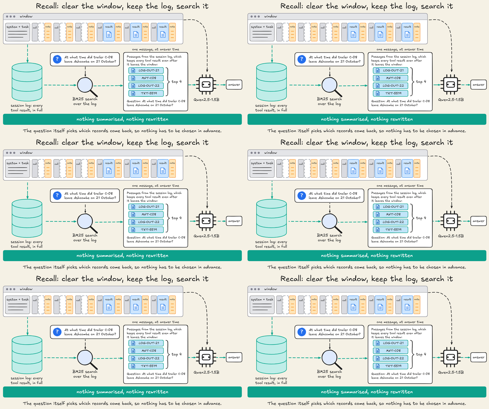
With the 1.5B reading, that policy answered 78 percent of the planted facts, against 63 percent for the full window.
That log held 137 passages from one investigation, and we searched it in memory, so Part 17 never asked what kind of store it needs.
A production agent writes to its log at every step of every session and searches it moments later, so the log is a write-heavy store.
Part 16 named synchronisation as the main operational cost of an index.
A revised document needs reprocessing, a deleted one must disappear from the index, and an access change must reach every stored copy.
This part asks whether those three changes are cheaper to carry with the vectors inside the database that already holds the data, or with a dedicated vector database beside it.
We start with what the default design leaves out and how a filter breaks a vector index, then compare four ways to store the vectors and five ways to keep them in step.
The hands-on then loads one million Wikipedia passages and the Halvern documents from Parts 13 to 15 and 17. Both go into Postgres with pgvector and into Qdrant, on one laptop.
It measures what search benchmarks show, the write load of an agent's memory, and how long search stays wrong after each kind of change, with seven injected faults.
With both indexes tuned, pgvector matched Qdrant's throughput at 0.95 recall against exact search, and Qdrant held its recall under narrow filters that follow content.
Under the injected faults, every wrong result came from a copy the commit's transaction did not update.
What the default design leaves out
The default design for a new retrieval system is an embedding model and a dedicated vector database.
Parts 1 to 4 followed it. Qdrant ran in Docker, and each chunk's vector went into a collection.
The chunk's text, or in Part 4 a summary of it, travelled with the vector in the point's payload. Every search result carried the passage to show the model.
For a corpus that is loaded once and then read, that design is sound.
In production, documents get revised, some have to be erased, and access to others is withdrawn.
One document, two copies
Each change lands first in the system that owns the data, usually a relational database such as Postgres. It then has to reach the copy in the vector store.
The copy holds the document's vector, its access groups, its version and, as in Parts 1 to 3, its text.
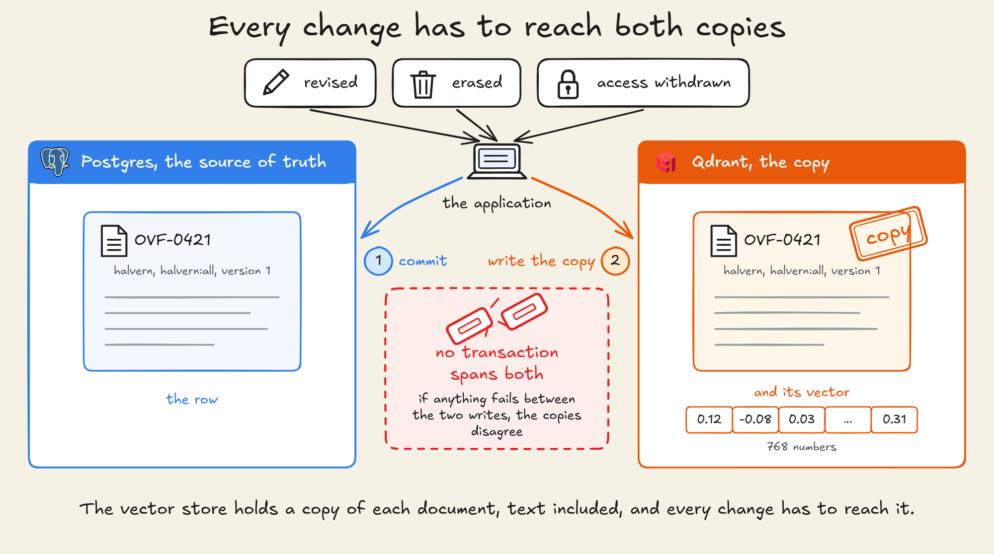
Dual-write means the application writes every change to both stores.
No transaction spans the two systems, so between the commit in the database and the write to the vector store there is always a gap.
The gap between two commits
Each of these failures leaves the two copies disagreeing, and neither store reports the disagreement:
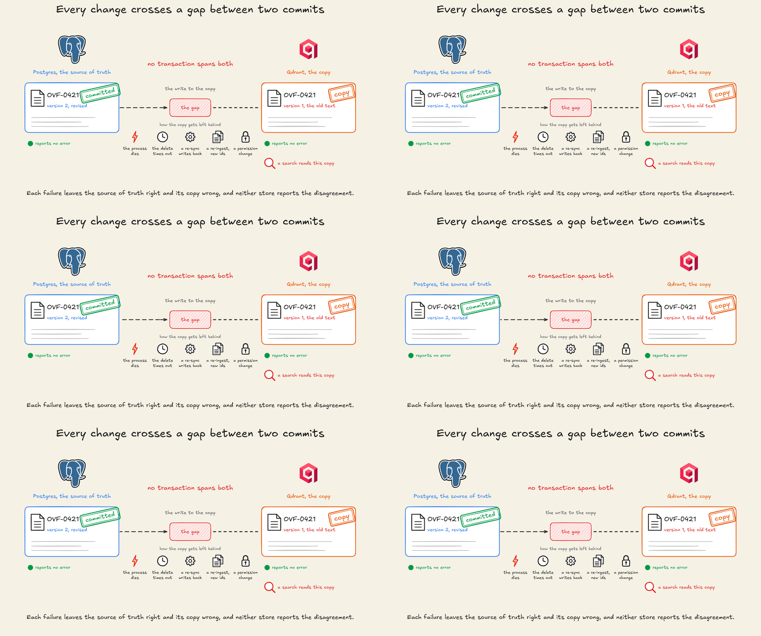
- In a partial write, the database commits and the process dies before the vector store hears of it.
- A delete can succeed in the database and time out in the vector store, which leaves an orphaned vector whose source row is gone.
- A re-sync job can read rows, embed them slowly and write them back over newer versions that landed in the meantime.
- A re-ingest without stable document identifiers adds a second copy of every document instead of replacing the first.
- A permission change can reach the source row and never the copy, so a group that lost access can still retrieve the document.
On Monday 2 November, Halvern's Dunmoor depot opens for the season. The overflow plan for Ashcombe's volume, OVF-0421, is revised to send overflow to Dunmoor instead of Northgate.
Suppose the revision commits in Postgres and never reaches the vector store.
A search for the overflow plan still returns the old note, text included. The model reading it is told that overflow goes to Northgate.
A stale embedding is a consistency failure between two copies of one document. The copy's vector still matches the old text it was built from.
Teams that ran vector search beside Postgres have written about moving it into Postgres. Keeping two stores in sync is one of the reasons they give.
Instacart's write-up (May 2025) describes replacing a standalone FAISS service with pgvector and says "storing data in two separate systems and keeping them in-sync led to inconsistencies".
Confident AI, which replaced Pinecone with pgvector (October 2023), listed synchronisation issues beside network latency, which it called the main bottleneck.
Three properties decide the store
Whether the second copy is worth its cost depends on three properties of the workload:
- Corpus size decides whether the vector index fits in the memory of the database the data already lives in.
- Write rate is how often the source of truth changes, set against how soon search must reflect each change.
- Filter selectivity is the share of the store that each query is allowed to see.
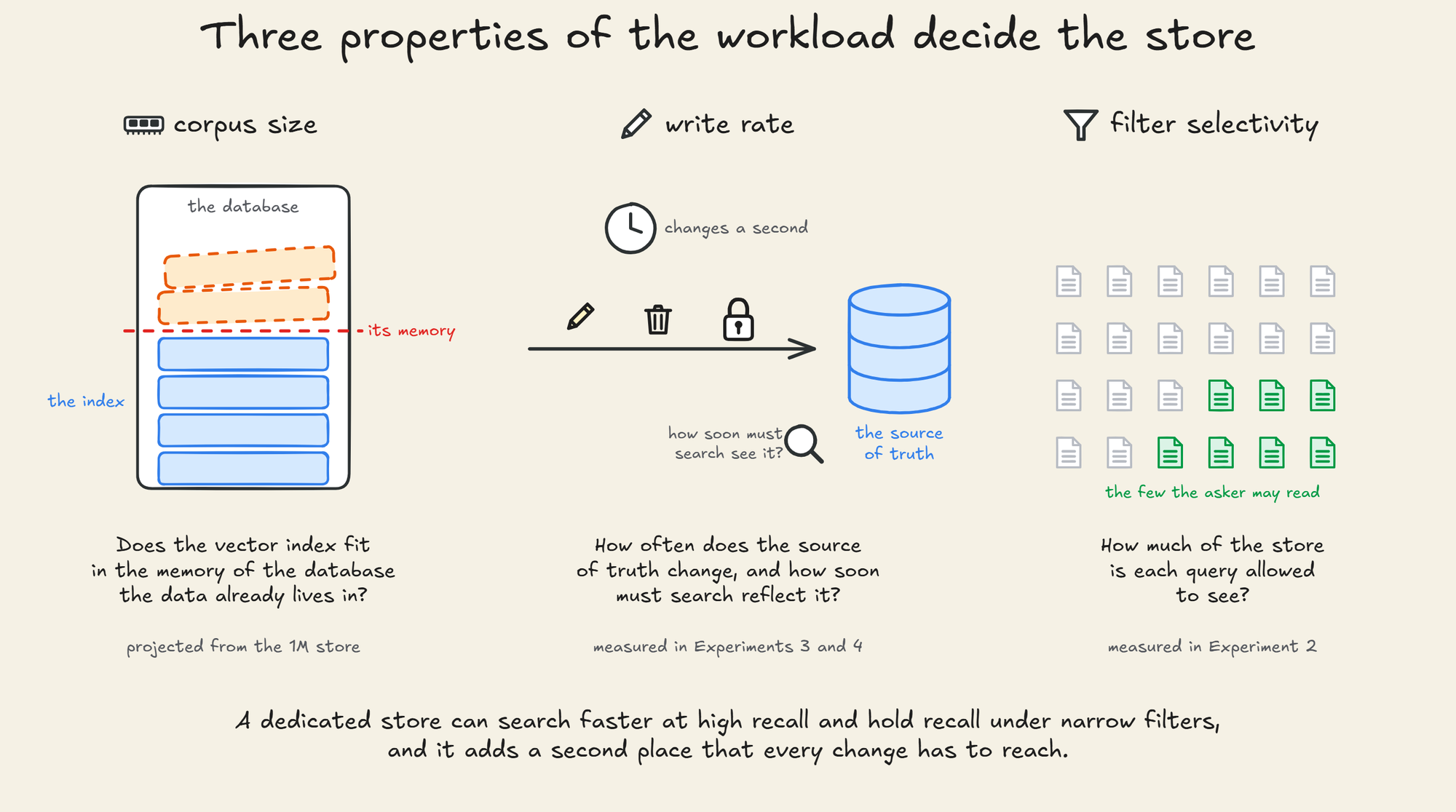
A dedicated store can search faster at high recall and hold recall under narrow filters. It also adds a second place that every change has to reach.
In the hands-on, we measure both sides on the same data.
How a vector index works, and where filters break it
Exact search, and why an index approximates it
The simplest vector search compares the query with every stored vector and keeps the closest ones.
It is always right, and its cost grows with the corpus. On our store, that is a million dot products over 768 dimensions for every question.
An approximate nearest neighbour index narrows the search to a small part of the store. A query is compared with thousands of vectors instead of all of them.
Part 1 introduced the idea, and Part 9 walked through HNSW, the graph index that both of our stores use.
The vector database guide linked from Part 9 covers it in full:
Avi Chawla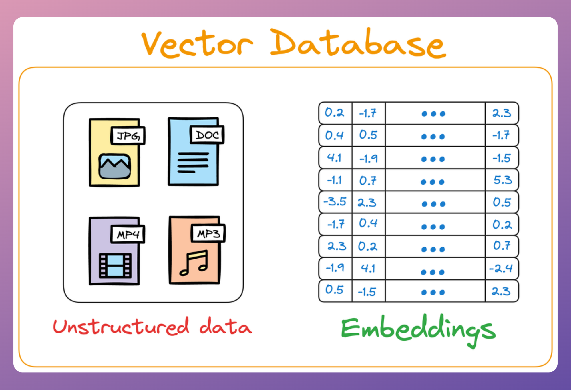
HNSW in one figure
HNSW, from Malkov and Yashunin's paper on hierarchical navigable small world graphs, links every vector to a few nearby vectors, in layers.
The bottom layer holds every vector. Each layer above it holds a smaller random share of the vectors below, so its links cover longer distances.
A search enters at the top layer and moves greedily, to whichever linked vector is closer to the query, until none is. It then drops one layer and carries on from where it stopped.
On the bottom layer, it keeps a list of the best candidates found so far and expands them in turn. It stops when no unexplored candidate is closer than the worst one on the list.
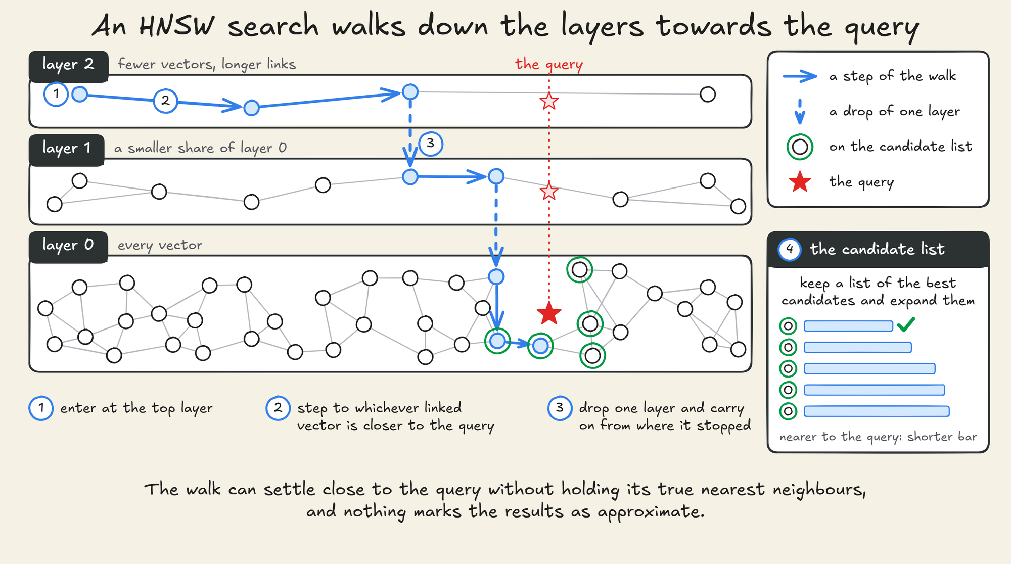
The walk can settle in a neighbourhood that is close to the query without holding its true nearest neighbours. Nothing then marks the results as approximate.
The settings that decide recall
Three numbers shape the graph and the search:
mis the most links each vector keeps per layer, and both stores allow twice as many on the bottom layer.- More links make the graph easier to navigate and the index larger.
- The build list (
ef_constructionin pgvector,ef_constructin Qdrant) is the candidate list used while the graph is built.- A longer list finds better neighbours to link, and the build takes longer.
- The search list (
hnsw.ef_searchin pgvector,hnsw_efin Qdrant) is the candidate list used while searching.- A longer list explores more of the graph and finds the true neighbours more often, for more distance computations per query.
The two stores ship different defaults:
m |
build list | search list | |
|---|---|---|---|
| pgvector 0.8.7 | 16 | 64 | 40 |
| Qdrant 1.20 | 16 | 100 | the build list's value, 100, unless set |
Of the three, the search list is the only one that can change from one query to the next without rebuilding the graph. It decides how far each search walks:
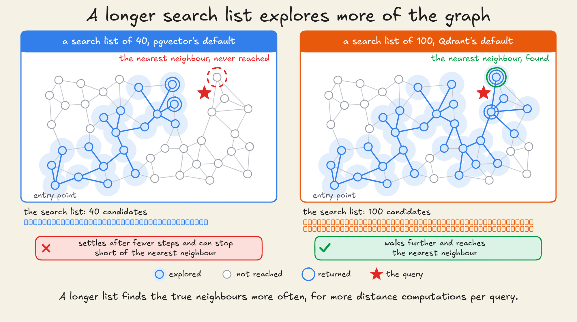
Every default sets a balance between speed and recall before the store has seen any data.
ann-benchmarks, the best-known benchmark for that balance, measures recall against exact search.
For each query, recall is the share of the true top 10 that the index returns.
Experiment 1 measures it for both stores, at their defaults and across a sweep of the search list.