When the Index No Longer Fits in Memory
Part 19: How much recall approximate search gives up once the vectors outgrow memory, measured against exact search at ten million vectors, with implementations
Recap
In Part 18, we put the same million Wikipedia passages into Postgres with pgvector and into Qdrant, and measured where each design holds up.
 Avi Chawla
Both stores lost recall at their defaults. pgvector found 84.0 percent of the true top 10 and Qdrant 94.4 percent, and a longer search list closed most of that gap.
Permission filters that follow content favoured Qdrant.
Changes favoured the designs that update everything search reads in one commit.
Part 18's decision map had three axes. The first, corpus size, applies to every design that keeps vectors. Past the sizes it marks, the map pointed to a smaller index, whose recall cost this part measures:
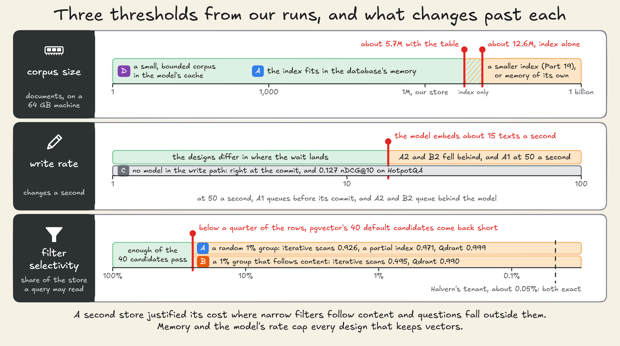
Part 18 stopped where the index still fits in one machine's memory at full precision.
This part uses Cohere's embeddings of MS MARCO web passages, 113.5 million in all, each with 1,024 dimensions.
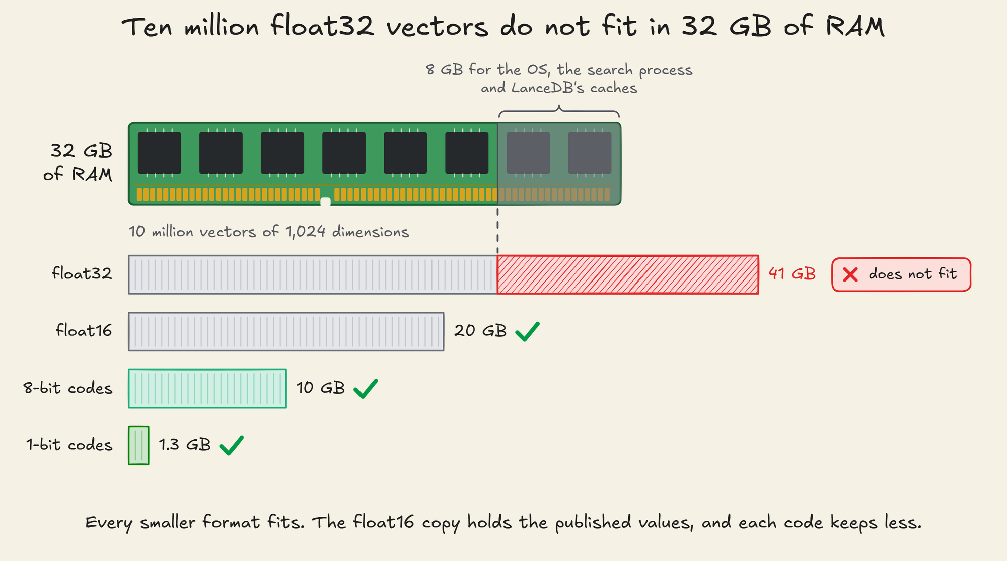
Ten million of them take 41 GB at float32, more than the 32 GB of RAM on the machine we measure on.
Cohere publishes them as float16, so a 16-bit copy holds the same values, but at 20 GB it leaves little room for an index beside it.
Every way of shrinking them further trades away recall, latency or both.
A result list does not show which true neighbours are missing.
This part measures that trade on 10 million real passage embeddings, for seven index designs:
- How much of the true top 10 each one returns.
- What that costs in latency once the full vectors sit on disk.
- How much memory an index needs before its latency holds.
- What appends and deletes do to an index built before them.
It then projects memory, build time, cost and latency to 100 million and a billion vectors.
Tuned to find 9 of the true top 10 on average, every design answered in 2.5 to 25.0 ms at the median with the full vectors on disk, as long as its index fit its cache.
What a vector costs in memory
Cohere's embed-english-v3 turns a passage into 1,024 numbers. Stored as 32-bit floats, that is 4,096 bytes.
A corpus multiplies that by the number of passages:
| Vectors | float32 | float16 | 8-bit codes | 1-bit codes |
|---|---|---|---|---|
| 1 million | 4.1 GB | 2.0 GB | 1.0 GB | 0.13 GB |
| 10 million | 41 GB | 20 GB | 10 GB | 1.3 GB |
| 100 million | 410 GB | 205 GB | 102 GB | 13 GB |
| 1 billion | 4.1 TB | 2.0 TB | 1.0 TB | 128 GB |
Our measurement machine has 32 GB of RAM. Leave 8 GB for the operating system, the search process and LanceDB's caches, and full-precision vectors stop fitting at about 6 million.
A float16 copy stops fitting at about 12 million, and Experiment 3 measures it.
At 10 million vectors, only the float32 copy overflows the machine's 32 GB:
Each index measured here stores a compressed code for every vector, plus a few bytes of bookkeeping or, for IVF-HNSW-SQ, its graph's links, and that is what has to live in RAM.
We measured what each design stores per vector, on the first 1 million passages of the corpus the hands-on uses:
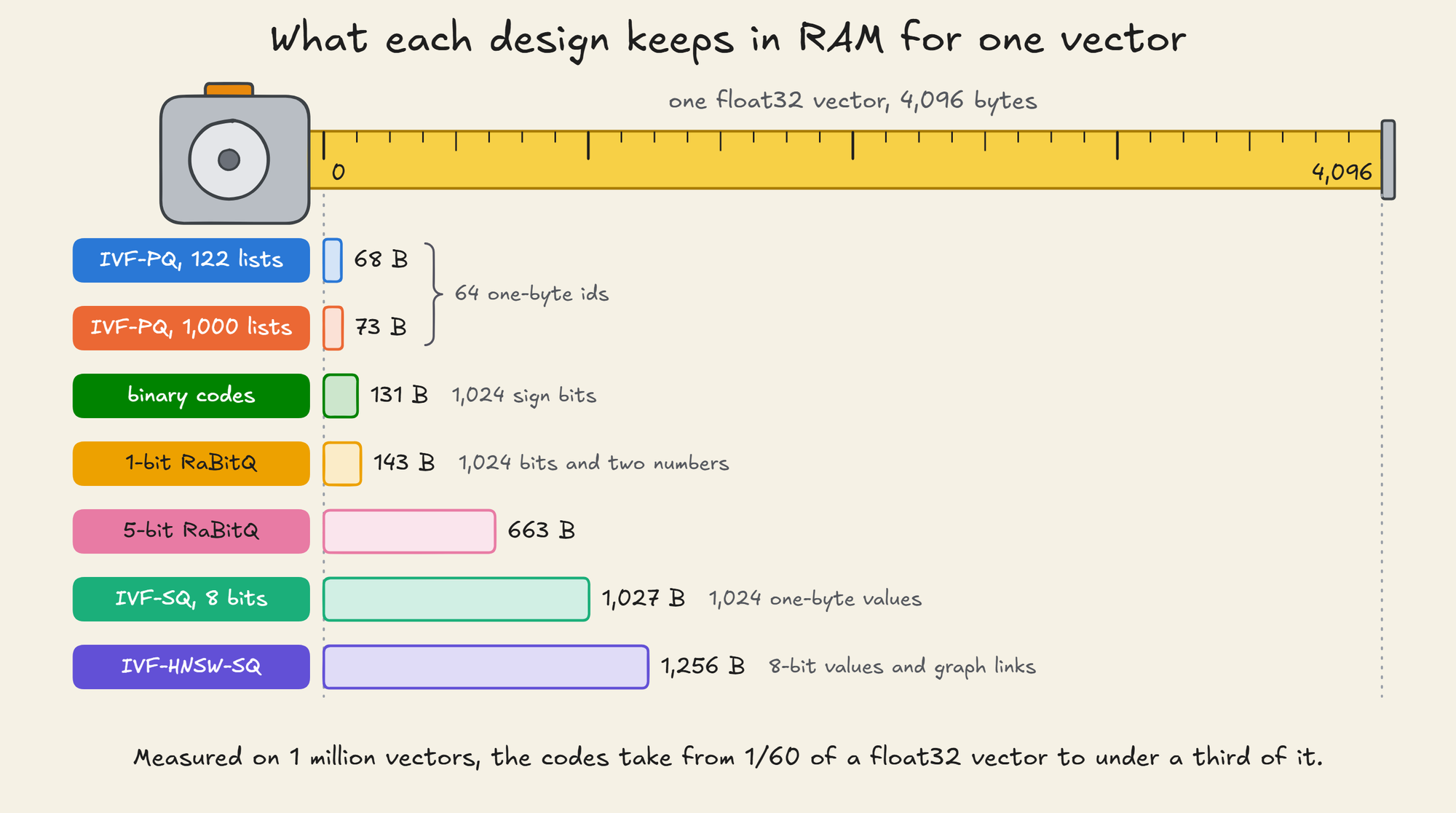
IVF-PQ, LanceDB's default index, stores 68 bytes a vector, and 73 with more lists. The 1-bit codes take 131 to 143 bytes, 5-bit RaBitQ 663, and 8-bit scalar codes 1,027.
An HNSW graph over 8-bit codes takes 1,256, because each vector also keeps links to its neighbours.
Apart from the graph's links, almost all of each number is the code itself: 64 bytes for PQ, 1,024 for the 8-bit codes, and 128 for 1,024 bits.
The rest is a few bytes of bookkeeping per row, plus small fixed tables that matter only at small sizes.
At 10 million vectors, the full float32 vectors are 41 GB. The PQ index takes 0.69 GB, and 1-bit RaBitQ's 1.45 GB.
The codes fit in RAM and the vectors do not, so every design splits into two parts that live in different places:
- The codes sit in RAM and decide which candidates a query can find.
- The full vectors sit on disk, and a query that rescores reads a few of them to rank its candidates by their true distance.
How approximate search buys speed
Exact search compares the query with every vector in the corpus.
At 10 million vectors, that is 10 million dot products over 1,024 dimensions, and every vector read for every query.
On our machine, LanceDB's exact search took a median of 303 to 331 ms a query at 100,000 vectors. At 10 million it took 58.1 s, with every query reading the vectors from disk.
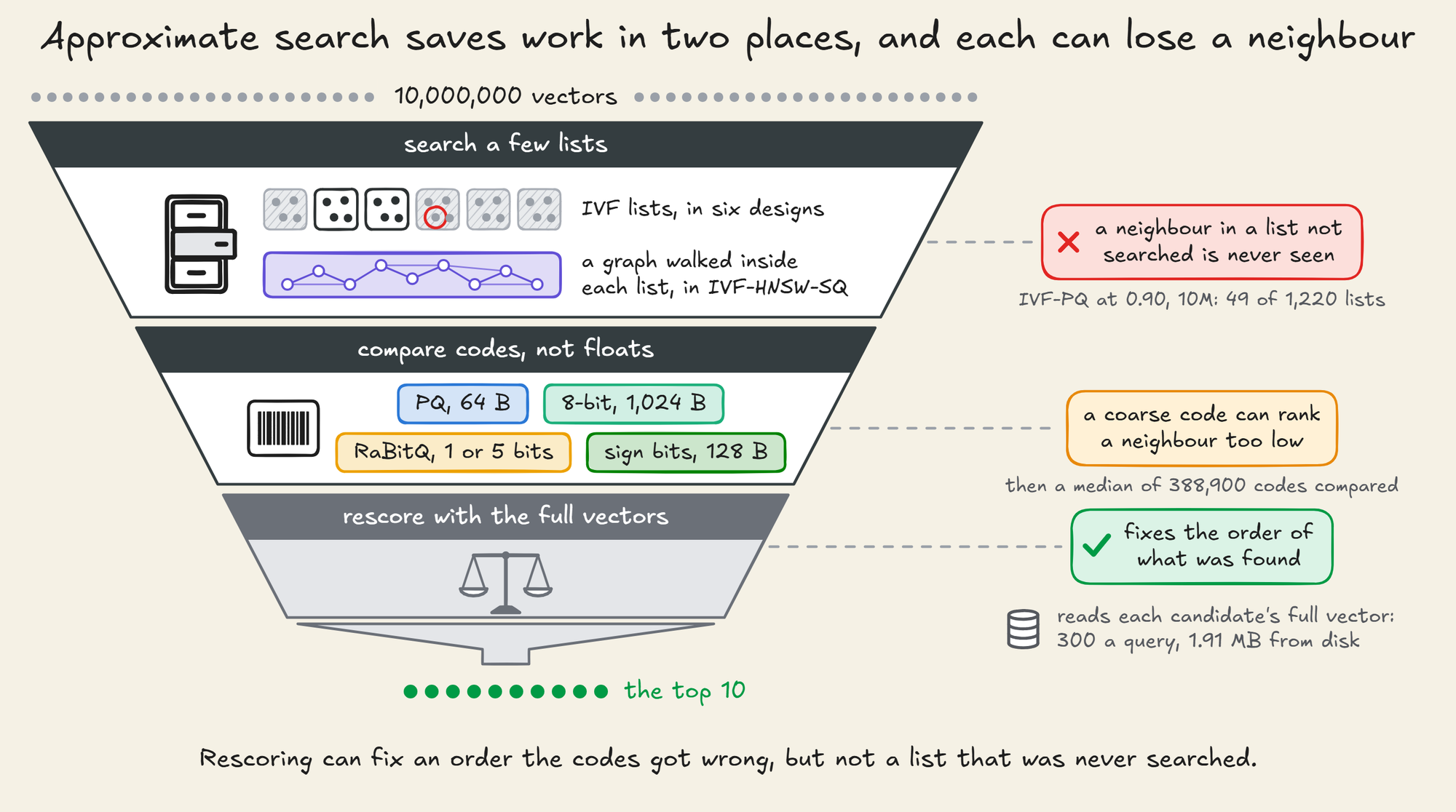
Approximate search cuts that cost in two ways.
It searches only part of the corpus, and it compares the query with compressed codes rather than with the full vectors.
The seven designs measured here combine the two in different ways:
Searching a few lists rather than all of them
An inverted-file index, or IVF, first groups the vectors.
It runs k-means over a sample of the corpus to find a set of centres, then files every vector in the list of its nearest centre.
LanceDB sets the number of lists from the size of the corpus:
- IVF-PQ and IVF-SQ get one list for about every 8,192 vectors, 1,220 at 10 million.
- RaBitQ and binary-code indexes get one for about every 4,096, 2,441 at 10 million.
- No index gets more than 4,096 lists.
A query first compares itself with the centres, which is cheap, then scans only the lists whose centres are closest:
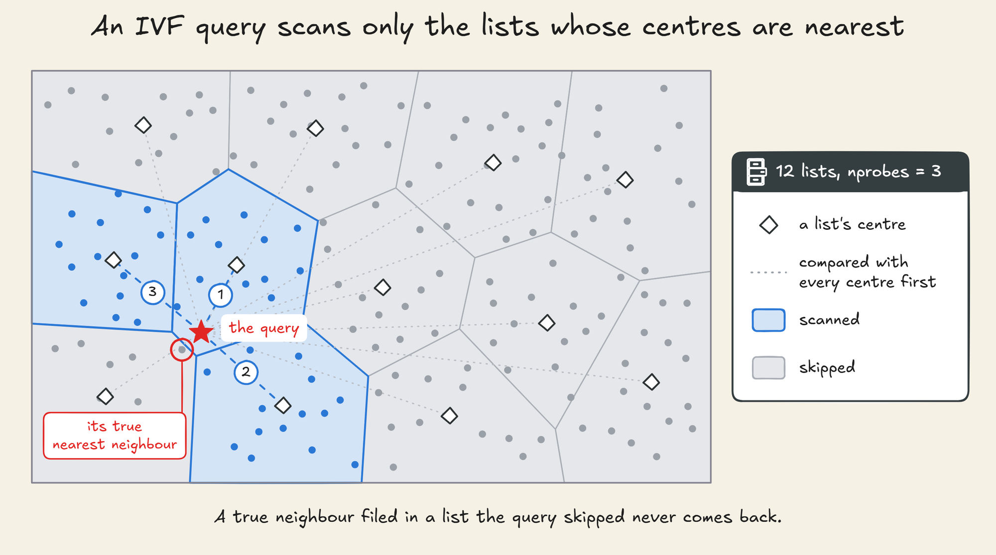
The number of lists scanned is the first knob. LanceDB calls it nprobes.
A true neighbour filed in a list the query did not scan is never seen at all.
Scanning more lists finds more of them, and every extra list costs a scan.
Product quantisation: 4,096 bytes down to 64
Scanning a list still means computing a distance to every vector in it, so the next cut is what each distance is computed against.
Product quantisation, a source-coding technique that Jégou, Douze and Schmid brought to nearest-neighbour search in 2011, cuts each vector into pieces and replaces every piece with the id of its nearest learned centre.
LanceDB's default takes each vector's offset from its list centre, as the paper's inverted-file version does, and cuts its 1,024 dimensions into 64 pieces of 16.
For each of the 64 positions it learns 256 centres with k-means, and it stores each piece as the one-byte id of its nearest centre:
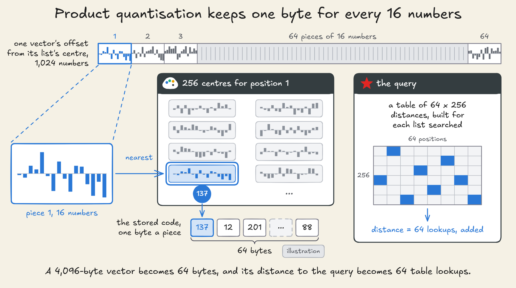
A vector becomes 64 bytes, 64 times smaller than its float32 form.
The distance is computed without decompressing anything.
For each list it searches, the query's offset from that list's centre is split the same way, and its distance to each of the 256 centres at each position goes into a table.
The distance to any vector in that list is then the sum of 64 table lookups.
The distance is approximate. Two vectors in the same list whose pieces round to the same centres look identical to the index, so a true neighbour can be ranked below a vector that only looks close.
Scalar quantisation, RaBitQ and binary codes
Scalar quantisation keeps every dimension and stores each value in 8 bits instead of 32. LanceDB scales every value into one range, from the smallest to the largest value in a training sample of 65,536 vectors, and clips anything outside it:
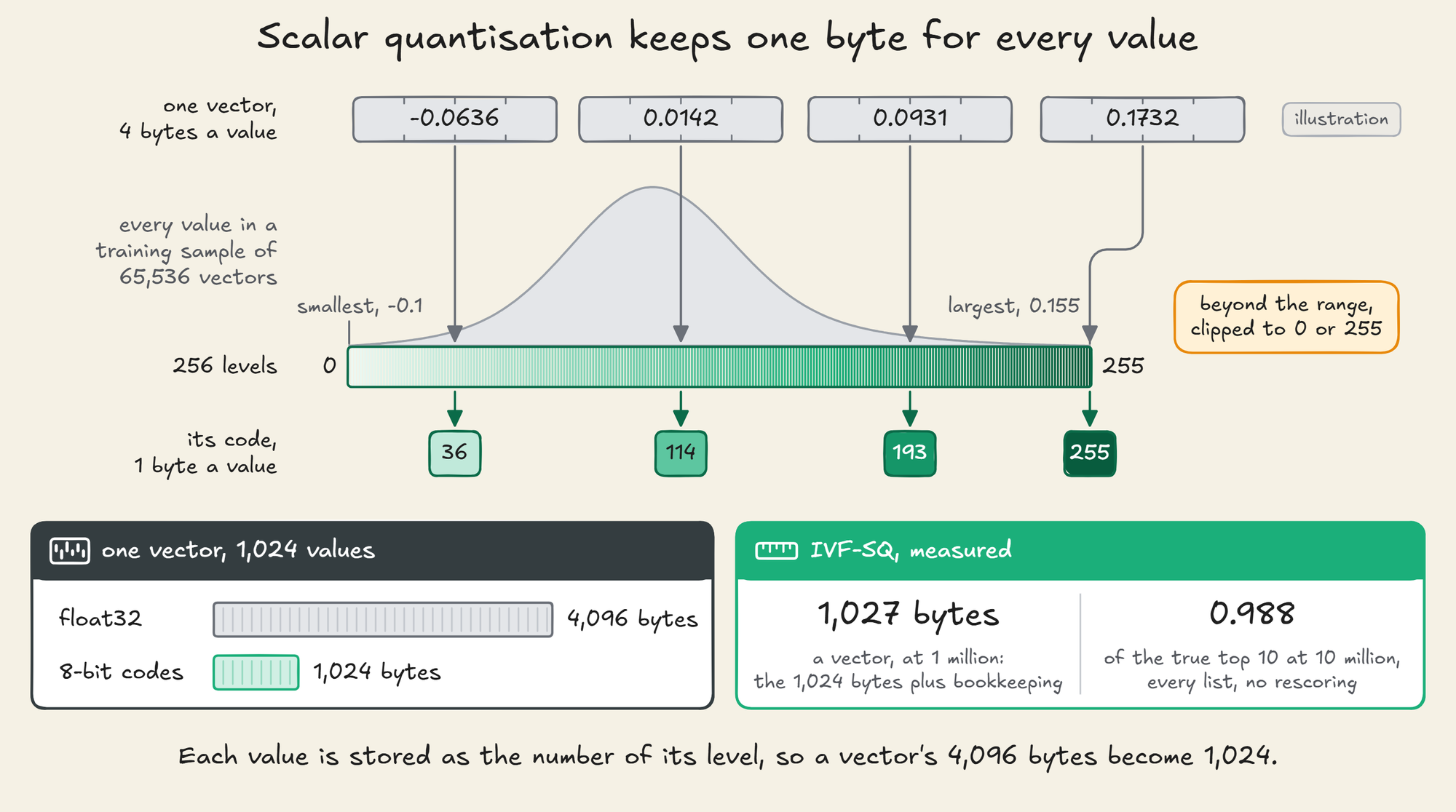
The code is four times smaller than float32, and its distances come much closer to the true ones than PQ's.
The smallest codes keep one bit per dimension.
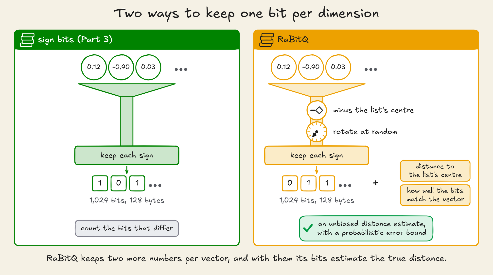
Part 3 used the simplest version: the sign of each dimension. A 1,024-dimensional vector becomes 128 bytes, and the distance between two codes is the number of bits that differ.
Comparing codes is cheap, and the distance is coarse.
So Part 3 searched for twice as many candidates as it needed, then ranked them again with the full vectors.
Part 3 also reported binary quantisation on about 32 million vectors in a private use case, with a speedup of about 35 times over a traditional RAG pipeline.
The DDS hands-on on binary quantisation builds a retrieval pipeline on these codes, step by step:
Avi Chawla
RaBitQ, from Gao and Long at SIGMOD 2024, also keeps one bit per dimension. It subtracts the list's centre and rotates the result at random before taking the bits, and stores two extra numbers per vector.
With those two numbers, its estimate of the squared distance is unbiased, and its error stays within a proven bound with high probability.
LanceDB's IVF_RQ index implements it, with 1 bit per dimension or, through the extended RaBitQ of 2025, more. Five bits is LanceDB 0.41's default.
Both start from the same vector, and RaBitQ adds two steps before it takes the signs:
A graph inside each list
HNSW, from Part 9 and Part 18, links every vector to its near neighbours and searches by walking those links towards the query, keeping a candidate list of size ef on the bottom layer.
LanceDB's IVF_HNSW_SQ, the last of the seven designs, builds one such graph inside each list, over 8-bit codes. Its default makes a list for about every million vectors, so at 10 million there are 9 lists of about 1.1 million vectors each.
A graph can be searched from disk. DiskANN, from Microsoft Research at NeurIPS 2019, showed that a graph kept on an SSD, with compressed vectors in RAM, can search a billion vectors on one machine with 64 GB of RAM.
LanceDB does not search its graphs on disk. It keeps them in the index files and loads a list's graph into an in-memory cache when a query first needs it:
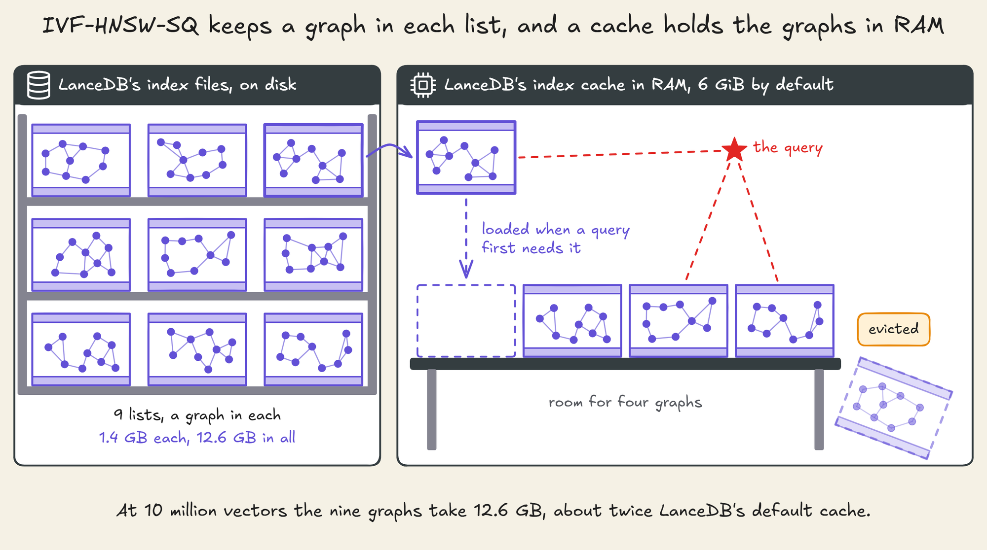
Experiment 3 measures how this design's latency depends on that cache.
Rescoring with the full vectors
Every code above computes an approximate distance, and rescoring repairs the ranking those distances produce.
The index returns its top k × R candidates by code distance. Their full vectors are read, the exact distances are computed, and the top k are kept.
LanceDB calls R the refine factor, and it is the oversample-then-rescore of Part 3 under another name.
With k of 10 and R of 10, the codes pick 100 candidates and their full vectors decide the final 10:
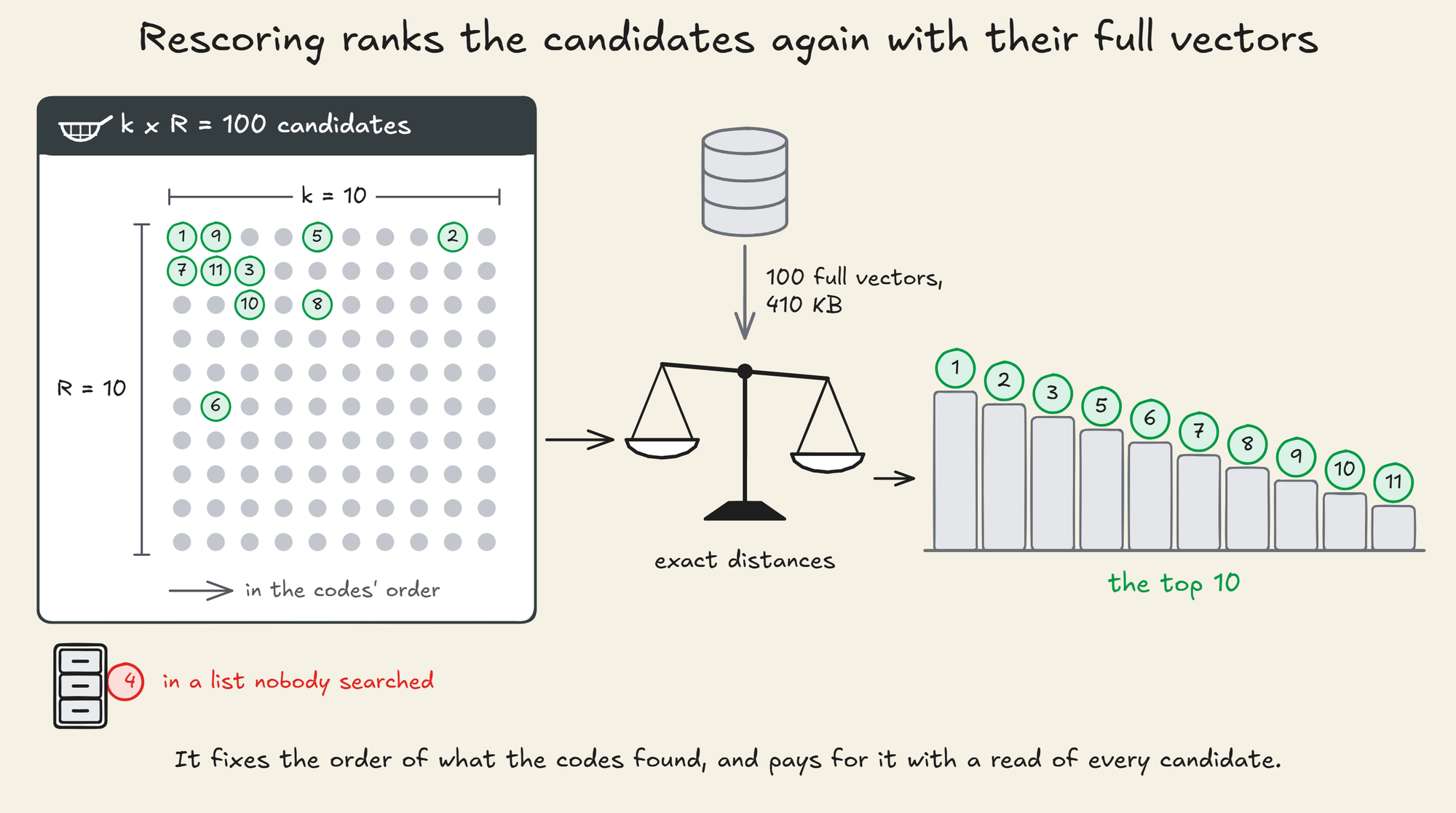
Rescoring fixes the order of the candidates the codes found.
It cannot recover a neighbour that sits in a list nobody searched.
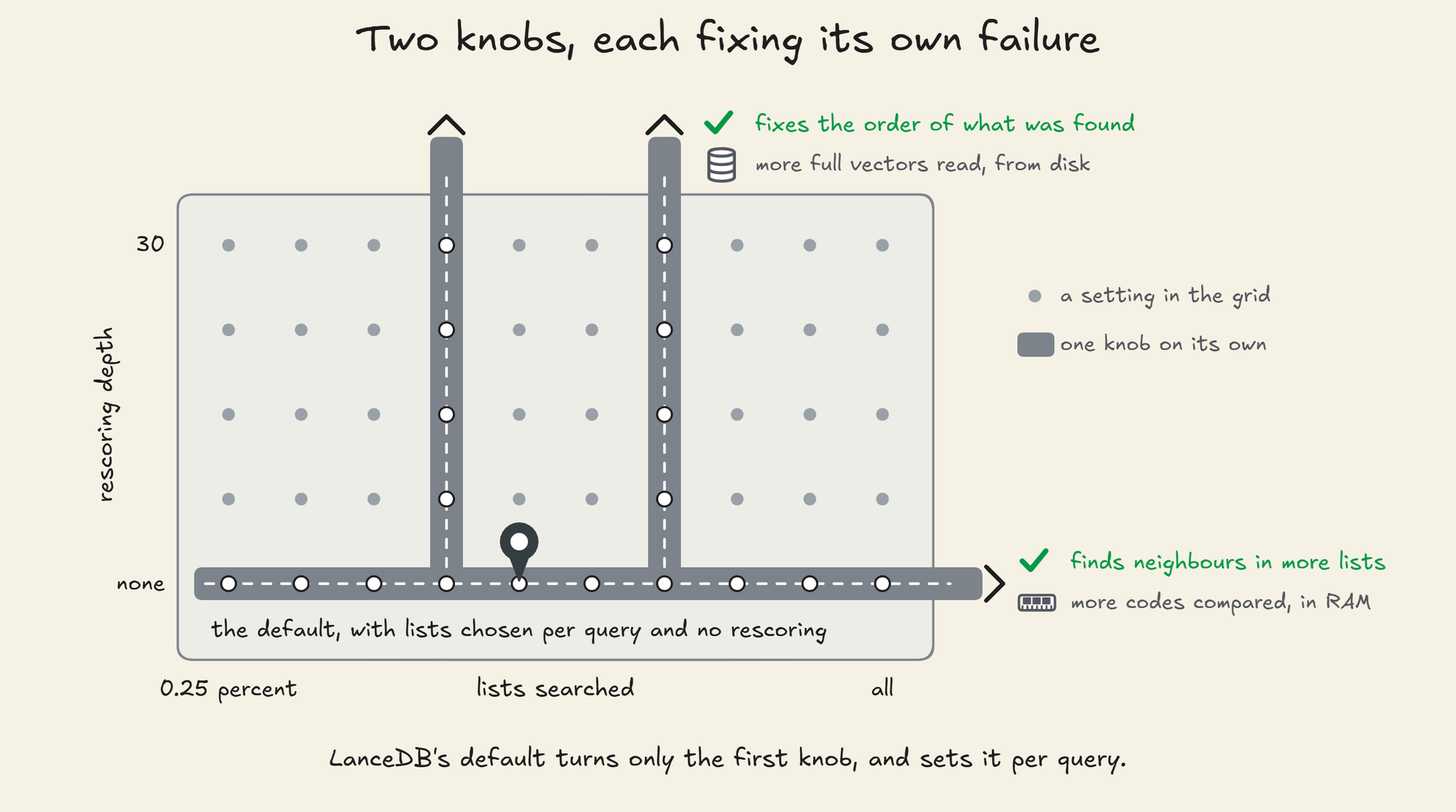
Lists searched and rescoring depth fix two different failures, and each has its own cost.
More lists mean more codes compared, in RAM.
More rescoring means more full vectors read, from disk once the vectors no longer fit.
What LanceDB does by default
The settings above are knobs, and a query that sets none of them gets LanceDB's defaults.
In LanceDB 0.41, the default query picks the number of lists for each query from how its distances to the list centres compare, taking every list whose centre is nearly as close as the nearest.
For a top-10 cosine query without a filter, that is never fewer than 8 lists or more than 77.
A setting called search_effort, 0.5 unless set, moves that number from one list at 0 to every list at 1.
On the PQ index at 1 million vectors, the default scanned a median of 33 of 122 lists, and anywhere from 8 to 77, its floor and its cap.
As the corpus grew, the default searched a smaller share of the lists:
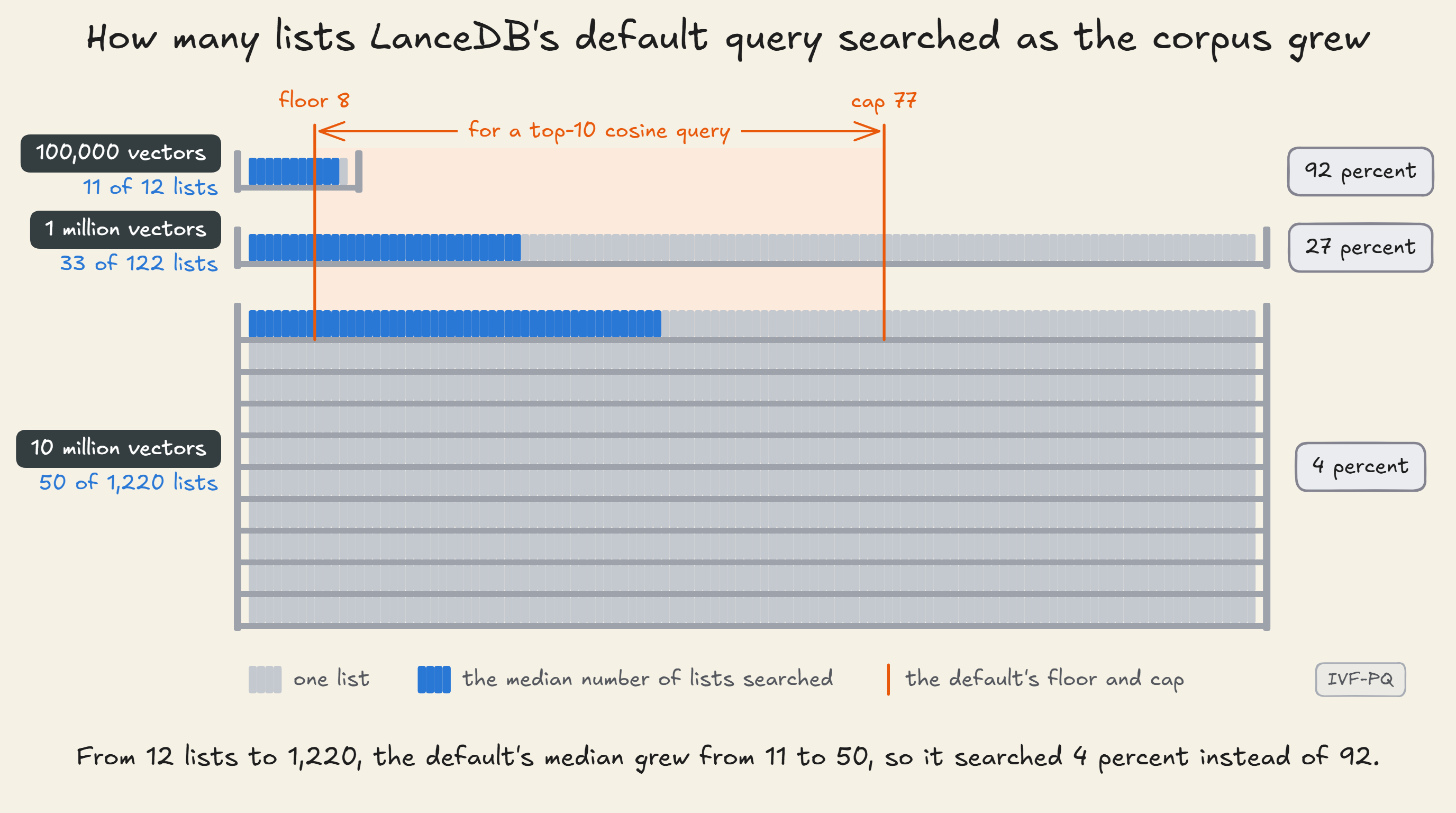
The default does not rescore. On IVF-HNSW-SQ, it searches each graph with an ef of 15, one and a half times k.
analyze_plan() instead of to_list(). It reports the lists searched and the codes compared, and the hands-on audits every setting this way.Together, the two knobs form a grid, and LanceDB's default sits on its bottom edge, with lists chosen per query and no rescoring:
Measuring what an index gives up
Recall is the share of the true top 10 that a query gets back. "True" means exact search over the same vectors, so the measurement needs the exact answer for every query first.
We use the 1,677 queries of the TREC Deep Learning tracks of 2021 to 2023, which come with Cohere's dataset, along with their own embeddings.
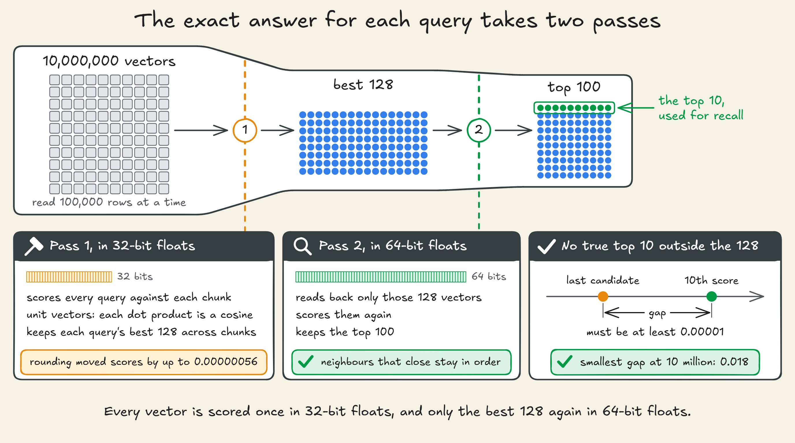
For each query, the exact answer takes two passes:
- Brute force over every vector of the corpus, in 32-bit floats, keeps the best 128 candidates.
- Those 128 are scored again in 64-bit floats, and the top 100 are kept.
32-bit rounding over 1,024 dimensions moved scores by up to 0.00000056 here. That is enough to swap two neighbours that sit that close, which is what the second pass prevents.
At 10 million vectors, the first pass scores every vector, and the second only the best 128:
The dataset carries its own exact search over all 113.5 million passages, which gives an independent check.
For 1,675 of the queries, the dataset's own top 1,000 includes a passage from our 10 million. For 1,673 of them, the best such passage is our exact top 1, and at 1 million all 1,505 agree.
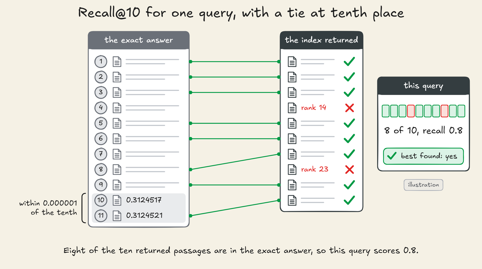
Two passages can sit at nearly the same distance from a query.
So the exact top 10 is widened to every passage whose true distance is within 0.000001 of the tenth, and a returned passage counts as correct if it is in that set, the rule big-ann-benchmarks uses.
For one query with a tie at tenth place, the count works like this:
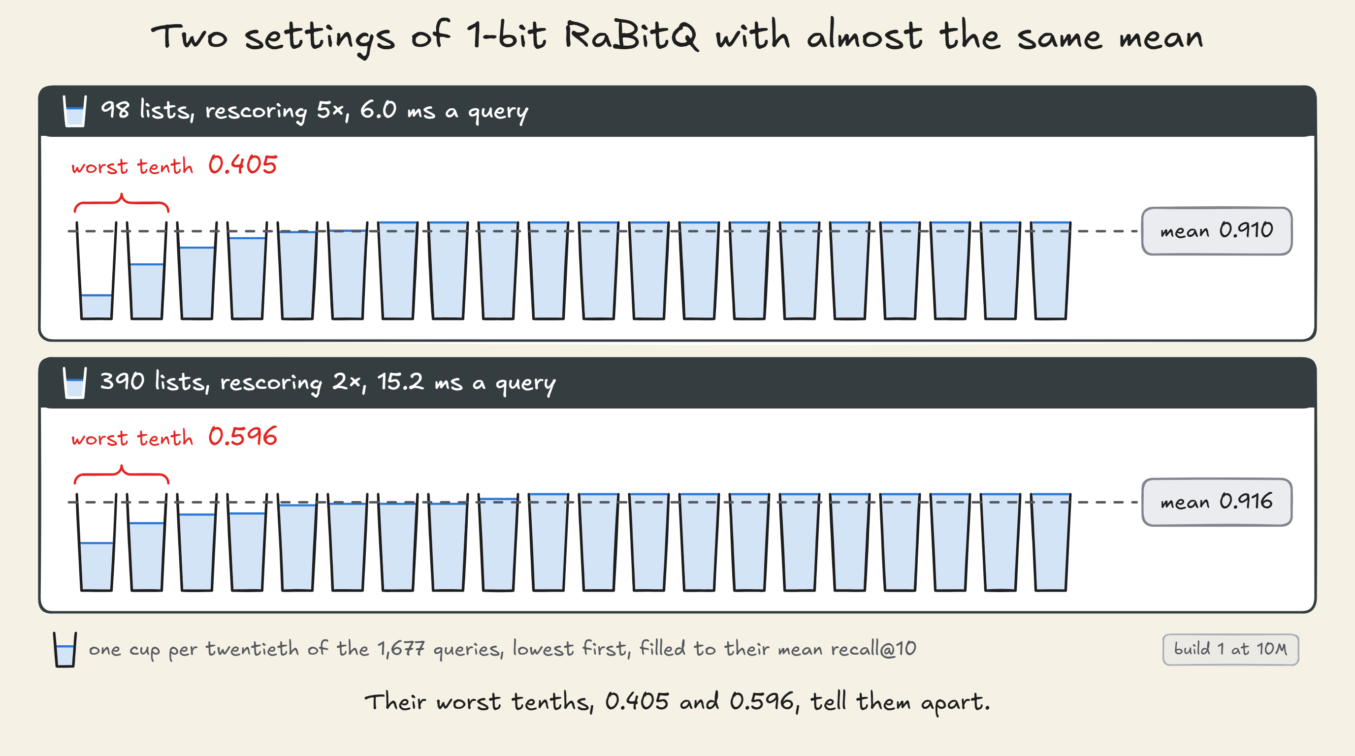
An average over 1,677 queries hides how the misses are spread. So every setting reports three numbers:
- Recall@10 is the mean over all queries.
- The worst tenth is the mean recall of the 10 percent of queries that did worst.
- Best found is the share of queries whose single closest passage came back at all.
For two settings of 1-bit RaBitQ at 10 million vectors, the mean barely moves and the worst tenth does:
An index built twice is not the same index. k-means starts from a random sample, and LanceDB exposes no seed for it, so every index is built three times.
The default and one-knob recalls are reported with their spread across the builds, and the grid runs on the first build alone.
Each knob is swept on its own first: lists searched, rescoring depth at about 2 and 16 percent of the lists, and LanceDB's own search_effort.
Then the full grid of lists against rescoring is walked, the way ann-benchmarks sweeps a grid of search settings for each index. A series stops once its recall stops rising.
For IVF-PQ with √n lists, the nine settings of a smaller pilot are timed as well.
To compare designs at the same quality, we take the fastest setting that reaches a mean recall of 0.90, the level at which the NeurIPS 2023 big-ann-benchmarks challenge ranked throughput, and separately 0.95. We call them each design's 0.90 and 0.95 points.
A point is chosen on half the queries, the tune half, where its mean recall must reach the target.
Experiment 2's table gives its recall on the held-out half, which the choice never saw, and the later experiments give it over all 1,677 queries. Latency is timed over all 1,677.
IVF-PQ's 0.90 point at 10 million vectors, chosen from all 53 settings Experiment 1 timed:
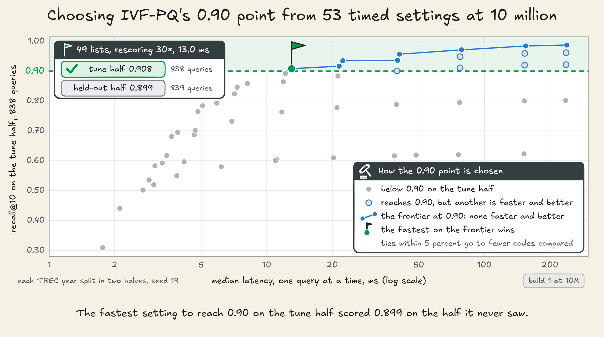
The two halves can disagree. At 100,000 vectors, IVF-SQ's chosen point reached 0.905 on the half that chose it and 0.890 on the half that did not.
From Experiment 2 on, latency is measured apart from recall, in a fresh process, at the chosen points, with 1, 8 and 32 clients at the 0.90 point.
It is measured in three states of memory, which the hands-on sets up and checks by the bytes each run read from disk.
Exact neighbours are not always relevant documents
Recall against exact search measures how much of the exact answer an index returns.
It says nothing about whether that answer is any good. The exact top 10 are the passages whose embeddings are closest to the query's, and the embedding model decides what close means.
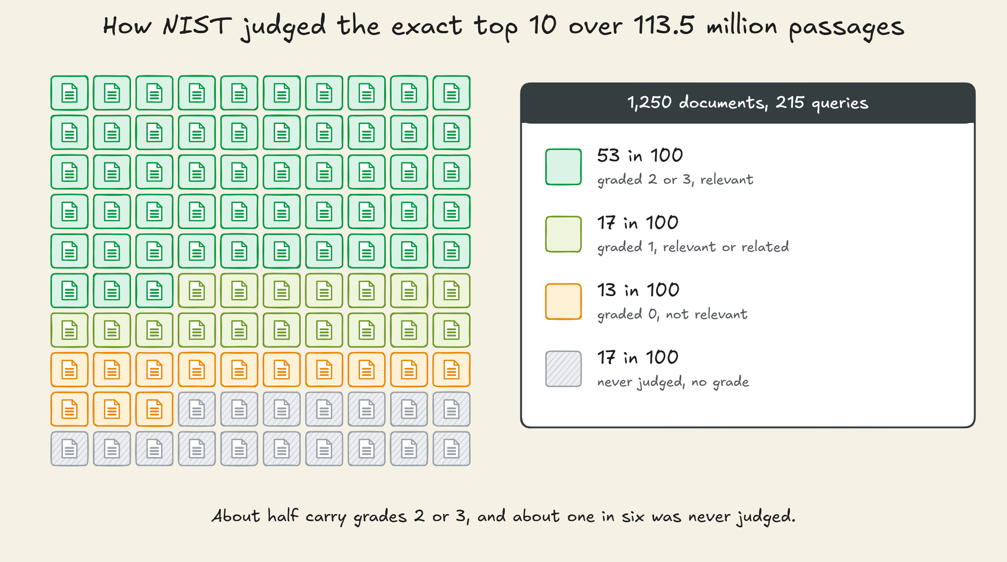
For 215 of the queries, NIST graded relevance on a four-point scale, from 0 for not relevant to 3 for perfect.
Its assessors graded documents for the 57 queries of 2021. For the 158 of 2022 and 2023 they graded passages, and each document's grade was inferred from its passages.
NIST counts document grades 1 to 3 as relevant. In 2022 and 2023, though, a 1 comes from passages it calls related but not relevant, so we also count grades 2 and 3 alone.
That gives a second measurement. Across the 215 judged queries, the exact top 10 over all 113.5 million passages hold 1,250 documents, with a document counted once when several of its passages appear.
The assessors had judged 82.7 percent of these documents. Of all of them, 69.9 percent carry grades 1 to 3, and 52.5 percent grades 2 and 3:
The same measurement on an index's answers, set against exact search over the same 10 million passages, asks whether its misses cost relevant documents.
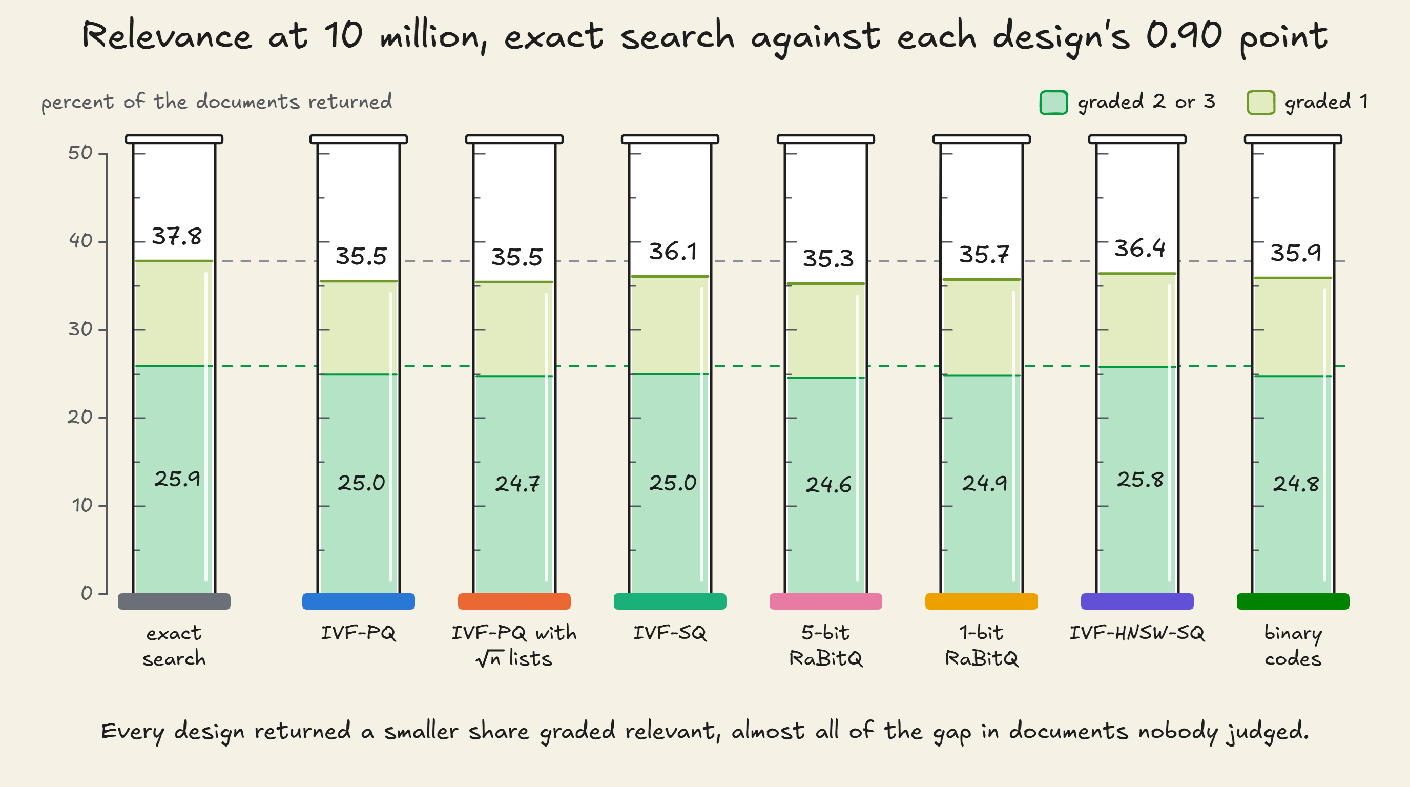
Over the first 10 million passages, exact search's top 10 holds a smaller share of judged documents, 49.4 percent, and 37.8 percent carry grades 1 to 3.
At each design's 0.90 point, 35.3 to 36.4 percent of the documents it returned carry grades 1 to 3, against 37.8 for exact search.
Counting grades 2 and 3 alone, the designs returned 24.6 to 25.8 percent, against 25.9 for exact search.
Almost all of each gap comes from documents the assessors never judged, which count as not relevant. The designs' answers held 45.8 to 47.0 percent judged documents, against 49.4 for exact search.
Among the judged ones, 76.6 to 77.6 percent carry grades 1 to 3, against 76.7 for exact search. So the test cannot say whether a design lost relevant documents, only that it returned more that nobody judged.
The shares graded 1 to 3 and graded 2 or 3, for exact search and for each design's 0.90 point:
Hands-on
Every measurement in this part comes from code in the zip, run over real embeddings apart from the control's random vectors.
The Halvern documents of the earlier parts number in the hundreds, and Part 18's Wikipedia passages stopped at a million.
Padding either to 10 million would need random vectors or millions of newly embedded passages. Random vectors' distances concentrate, and the control at the end of the experiments measures what that does to recall.
So the corpus is Cohere's embeddings of MS MARCO v2.1's segmented passages, published with their queries on Hugging Face. Indexing them needs no embedding bill.
Its 1,677 queries come with their exact top 1,000 over all 113.5 million passages, and 215 of them with NIST's relevance judgements, so both the exact answer and the relevant documents can be checked.
The embeddings are licensed under Apache 2.0. The passage text and NIST's judgements keep MS MARCO's terms, which allow non-commercial research only.