Why RAG Latency Is a Prefill Problem, Not a Retrieval Problem

Recap

Over the last twelve parts of this RAG systems course, we built RAG systems from the ground up.

• In Part 1, we assembled a complete pipeline. Documents were chunked, embedded, and stored in a vector database. A user query was embedded, matched against that store, and the retrieved chunks were passed to an LLM.
• Part 2 covered evaluation. We measured faithfulness, answer relevance, and context precision, and learned that a RAG system without measurement is a system nobody can improve.
• In Part 3, we tackled latency. We rebuilt the pipeline in a modular form, then applied binary quantization to compress vectors. Retrieval got roughly four times faster in our demo.

That work was correct. But it only targeted half of the latency problem in a RAG system.

More specifically, we measured how long retrieval took. We never measured how long the model took to read what retrieval returned.

In this chapter, we will be exploring why the prefill stage dominates RAG latency. We'll understand how the key-value cache works, why the standard fix (prefix caching) recovers almost nothing for RAG workloads, and what actually does work. As always, every notion will be explained through clear examples and walkthroughs to develop a solid understanding.

Let's begin!

Understanding a RAG pipeline from a latency perspective

Take a standard RAG request and break its latency into stages.

• Embedding the query takes a few milliseconds.
• Approximate nearest neighbor search over a few million vectors takes tens of milliseconds.
• Reranking eight candidates with a cross-encoder takes perhaps a hundred milliseconds.

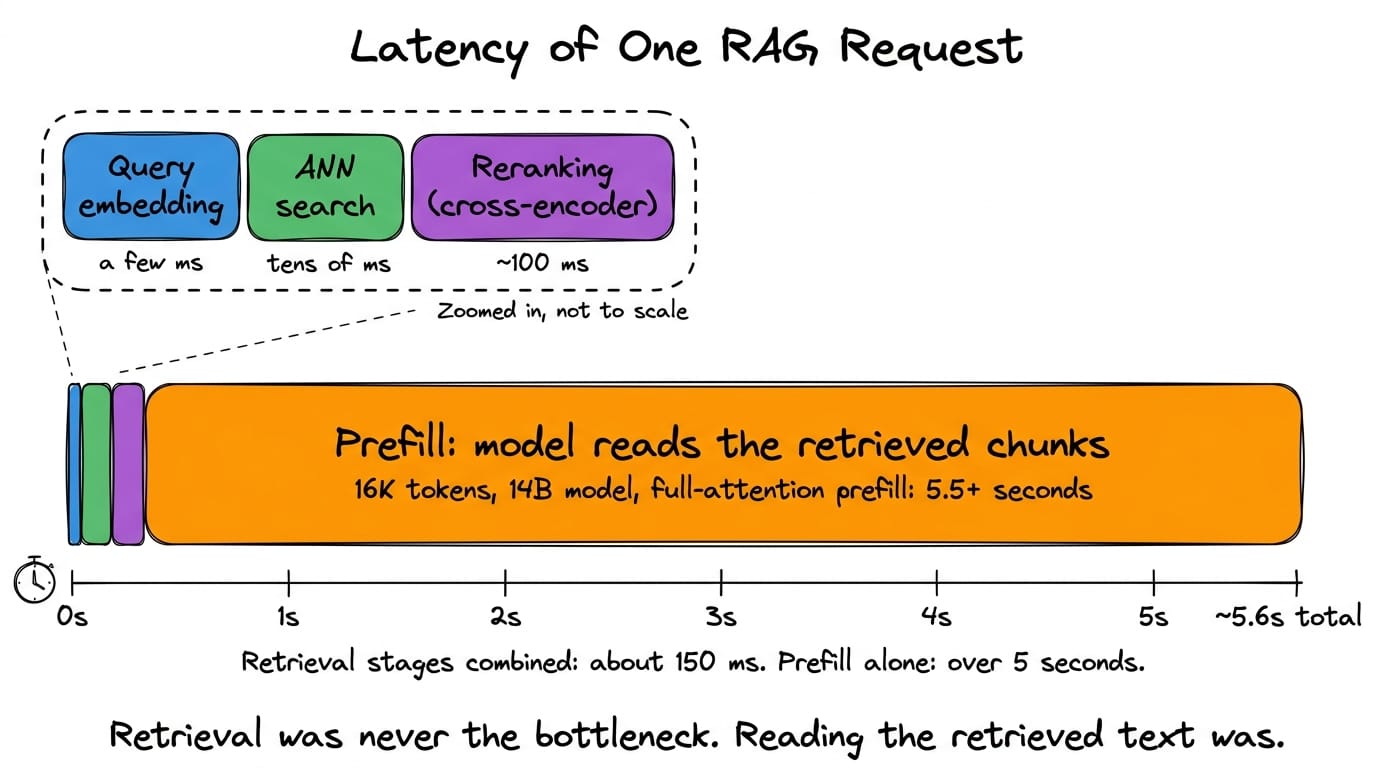
Then the model reads those eight chunks. That step, on its own, can take seconds.

Production RAG queries typically feed between four thousand and sixteen thousand tokens to the model, and most of that volume is retrieved text rather than the user's question.

At the higher end of context usage, the cost becomes severe. Processing sixteen thousand input tokens with a fourteen billion parameter model on an NVIDIA L20 GPU has been measured at over five and a half seconds before a single output token appears, under full-attention prefill:

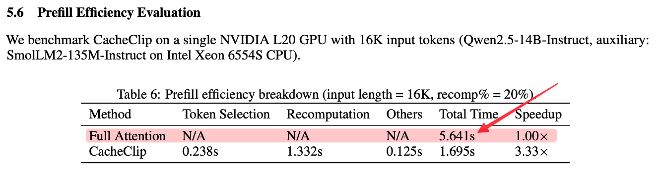
When the LLM reads the text, it's a bigger bottleneck than retrieval.

This reframes what "optimizing RAG" means. Part 3 saved milliseconds off a stage that was already cheap. The expensive stage sat directly downstream:

There is a reason this stage is expensive, and a reason the obvious fix does not work. Both come from the same place, which is how transformers actually process input. So let's discuss it next.

Prefill and decode are two different mechanisms

Autoregressive generation happens in two phases with opposite performance characteristics. And most confusion about inference latency comes from treating them as one thing.

The prefill phase

When a request arrives, the model must first read the entire input. It processes every token in parallel through every layer, computing attention across the full sequence.

During this pass, each layer produces two tensors for every token. These are the keys and the values, the quantities attention uses to decide what to look at and what to retrieve from. Together, they are stored as the key-value cache, usually shortened to KV cache.

Prefill is compute-bound. The attention computation scales with the square of the sequence length, because every token attends to every preceding token. So doubling the input quadruples the attention work.

It is worth making that quadratic term explicit, because it is the reason retrieved context is expensive rather than merely large.

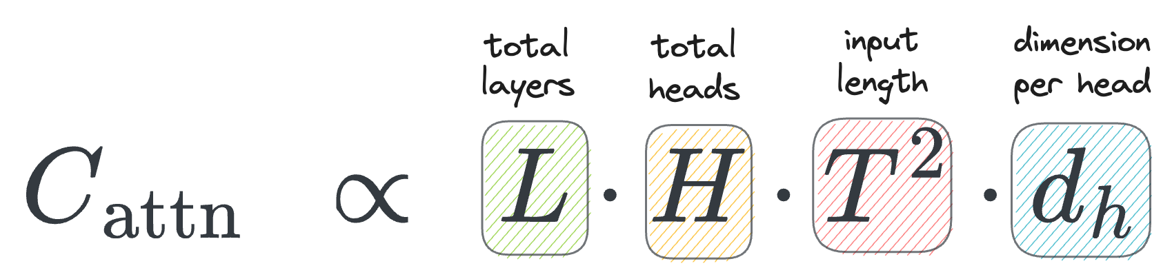
Reading the symbols:

• $C_{\text{attn}}$ is the attention compute for one prefill pass
• $L$ denotes the total number of layers
• $H$ denotes the total number of heads
• $T$ represents the input length in tokens
• and $d_h$ is the per-head hidden dimension.

The proportionality hides any constant factors that depend on hardware and kernel implementation.

Structurally, the term that dominates the computation equation below is $T^2$:

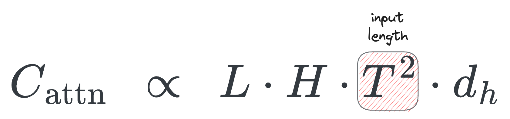
Every one of the $T$ query vectors forms a dot product against every one of the $T$ key vectors, which produces a score matrix with $T^2$ entries.

That matrix is built independently in every head of every layer, which is where $L$ and $H$ enter as multipliers.

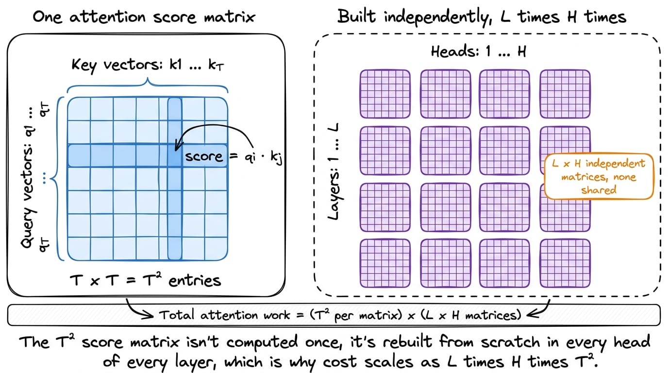
The intuition is that context length is the expensive dimension, and it is expensive in a way that compounds.

Going from 2,000 tokens to 4,000 does not double the attention cost but rather roughly quadruples it. Adding a ninth retrieved chunk to a prompt that already holds eight costs more than the first chunk did, because the new tokens must attend to everything already present and everything present must now account for them.

This is why RAG changed the economics of serving.

A bare question is a few dozen tokens. The same question with eight retrieved passages attached can easily become several thousand tokens instead, and the attention cost moved by a factor far larger than eight.

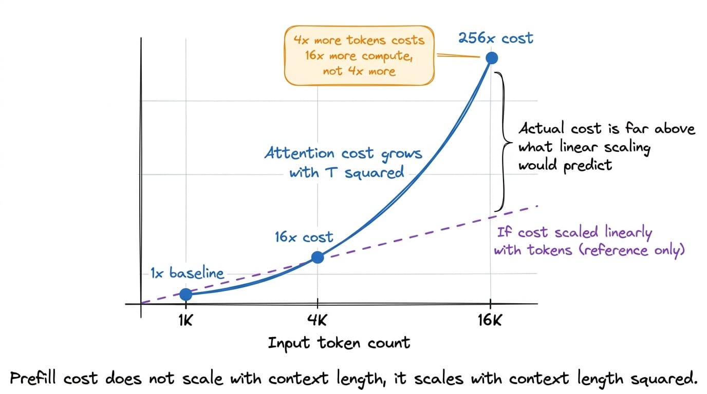
The time this phase takes is what the user experiences as the delay before the first word appears. The standard name for it is time to first token, or TTFT.

The decode phase

Once prefill finishes, the model generates output one token at a time. Each new token attends to everything before it, which is exactly what the stored KV cache holds.

Because the cache already exists, decode never recomputes attention over the input. It computes keys and values for one new token, appends them to the existing KV cache, and the process continues to subsequent tokens as they are generated.

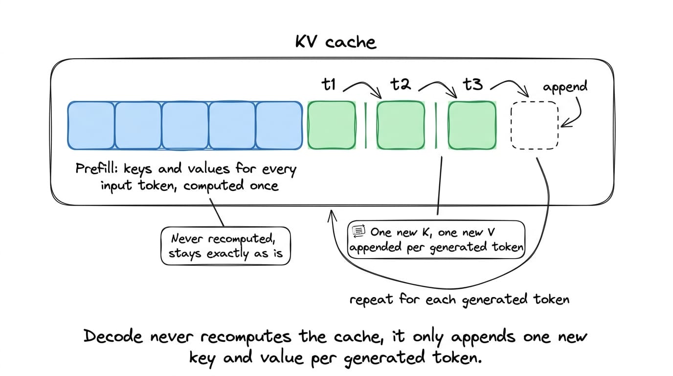
Decode is memory-bandwidth-bound rather than compute-bound. Each step must stream the model's weights from memory to produce a single token, so the hardware spends most of its time waiting for weights transfer rather than actually running the computation to predict the next token.

The asymmetry is important to understand because it explains why the two phases respond to completely different optimizations.

• During prefill, thousands of tokens flow through the same weights at once, so the cost of loading those weights is spread across thousands of useful calculations.
• During decode, the identical weight loading happens to serve one token.

A seven billion parameter model in fp16 precision holds roughly 14 GB of weights. Producing a single decode token requires reading essentially all of them.

The arithmetic performed against those weights is tiny by comparison, which means the accelerator sits idle waiting on memory for most of the step.

This is the reason batching helps decode (the second stage) so much and helps prefill (first stage) comparatively little.

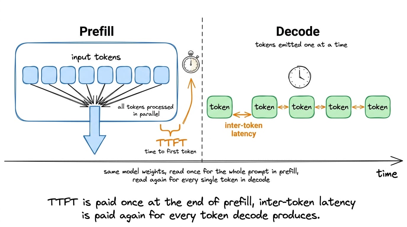
During decode, the expensive step is reading the model's weights from memory, and that read produces only one token. Batching sixty-four requests together reuses a single weight read to produce sixty-four tokens at once (because there are sixty-four requests being served in parallel), so the cost is shared across all of them instead of being paid per token.

Prefill gets little from this mechanism, because a single request already pushes thousands of tokens through those weights at once and keeps the hardware busy.

For this article, only a small part of that matters. Optimizing decode is a different discipline with different tools. RAG's latency problem is concentrated in prefill, and prefill responds to exactly one thing, which is not repeating the computation you have already computed.

What the cache actually costs

The KV cache is not free. Understanding its size tells us why reusing it matters so much, and later, why storing many versions of it becomes a problem.

The memory a cache occupies grows with the sequence length, the model depth, and the width of each attention layer.

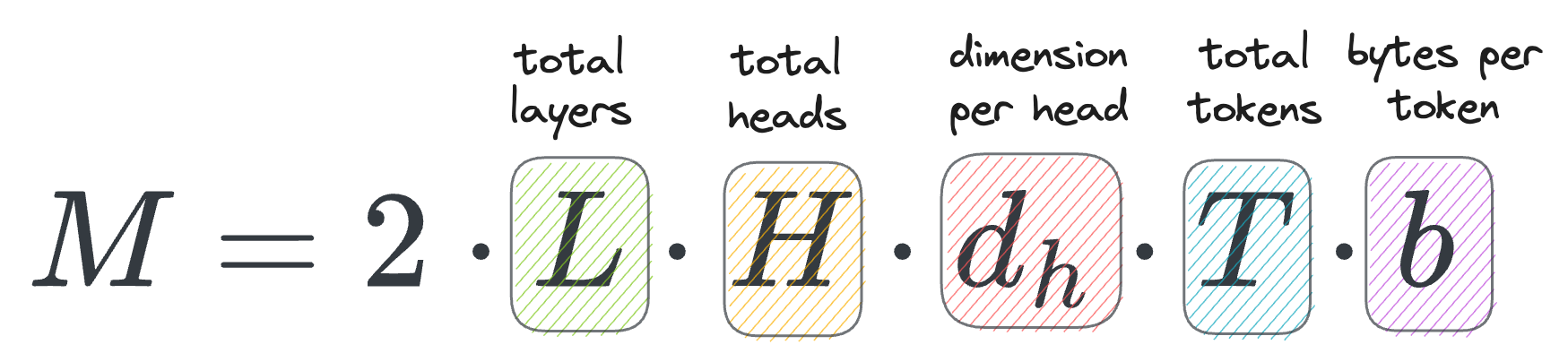
Every symbol here is straightforward

• $M$ is the total memory in bytes.
• The leading factor of $2$ accounts for storing both keys and values (and they are of equal length/size).
• $L$ is the number of transformer layers, since every layer keeps its own cache.
• $H$ is the number of attention heads per layer and $d_h$ is the dimension of each head.
• $T$ is the number of tokens currently cached
• Finally, $b$ is the bytes per element, which is $2$ bytes for half precision (fp16).

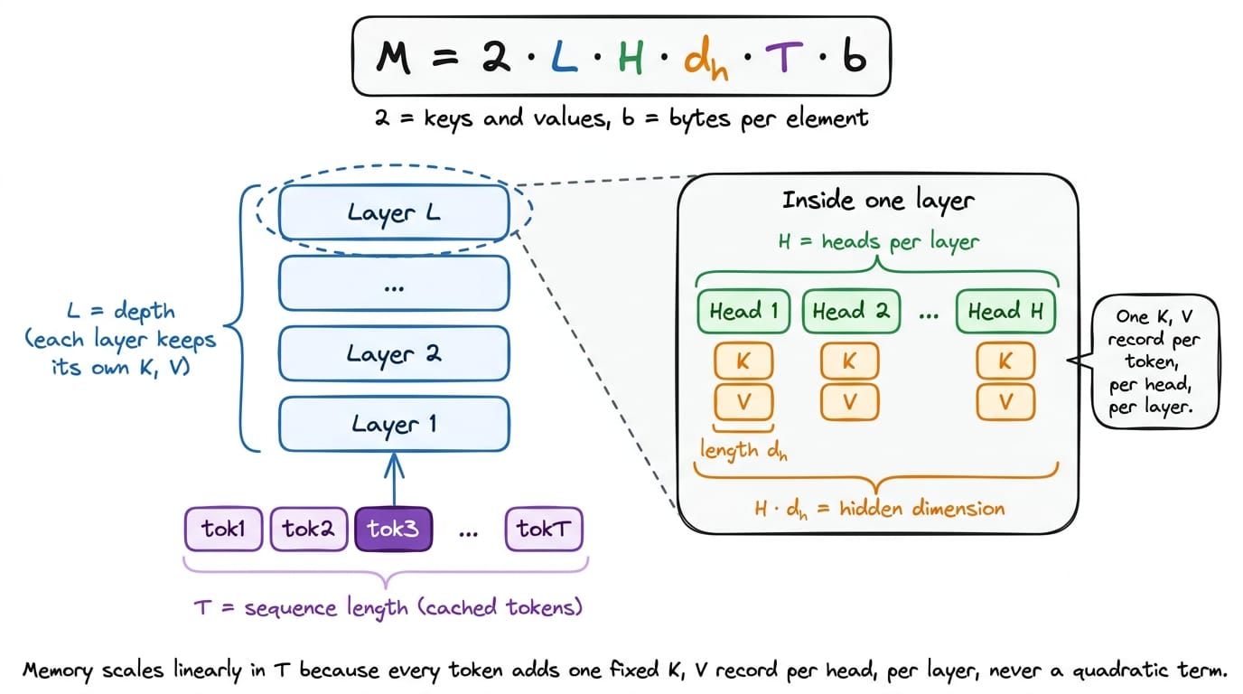
Reading the structure, the product $H \cdot d_h$ is simply the model's hidden dimension spread across heads. Multiplying by $L$ accounts for depth. Multiplying by $T$ makes the whole thing linear in sequence length, which is the important property.

Do note that, unlike attention compute, cache memory does not grow quadratically.

The intuition is that the cache is a per-token record, kept once per layer, for both keys and values. Every additional token of context adds a fixed cost. Every additional layer multiplies it. A model twice as deep needs twice the cache for the same input.

Let's work on an example to make this concrete.

Consider a model with 32 layers, 32 heads, and a head dimension of 128, holding 8,000 tokens in half precision.

This would need roughly 4 GB of cache for a single request. It is important to note that this memory will be unavailable to any other request while it is held by this specific request.

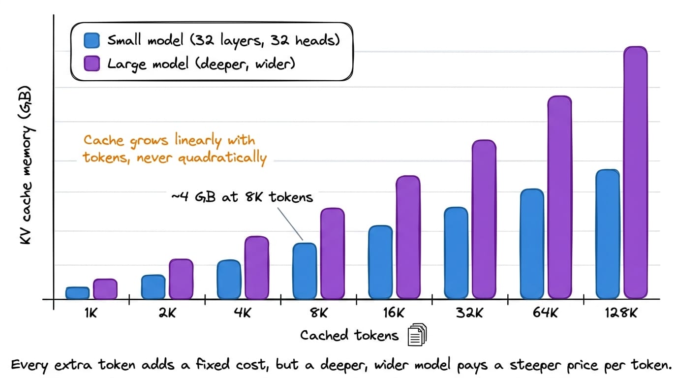
In summary, prefill pays a large one-time compute cost and produces a cache. The decode process then consumes that cache cheaply.

If we could avoid paying the prefill cost repeatedly for text we have already processed, RAG latency would improve substantially. That idea is what prefix caching implements.

How prefix caching works

Serving engines already reuse KV caches across requests. Understanding exactly how they do will let us see, precisely, why the mechanism underperforms for RAG.

Paged memory for the cache

Early serving systems allocated one contiguous memory block per request, sized for the longest output the request might produce. Most requests finished early, so most of that memory sat unused.

The PagedAttention design, which underlies vLLM, borrowed the solution from operating systems. Instead of contiguous per-request buffers, the cache is split into fixed-size blocks that can live anywhere in memory. A request holds a list of block references rather than one large region.

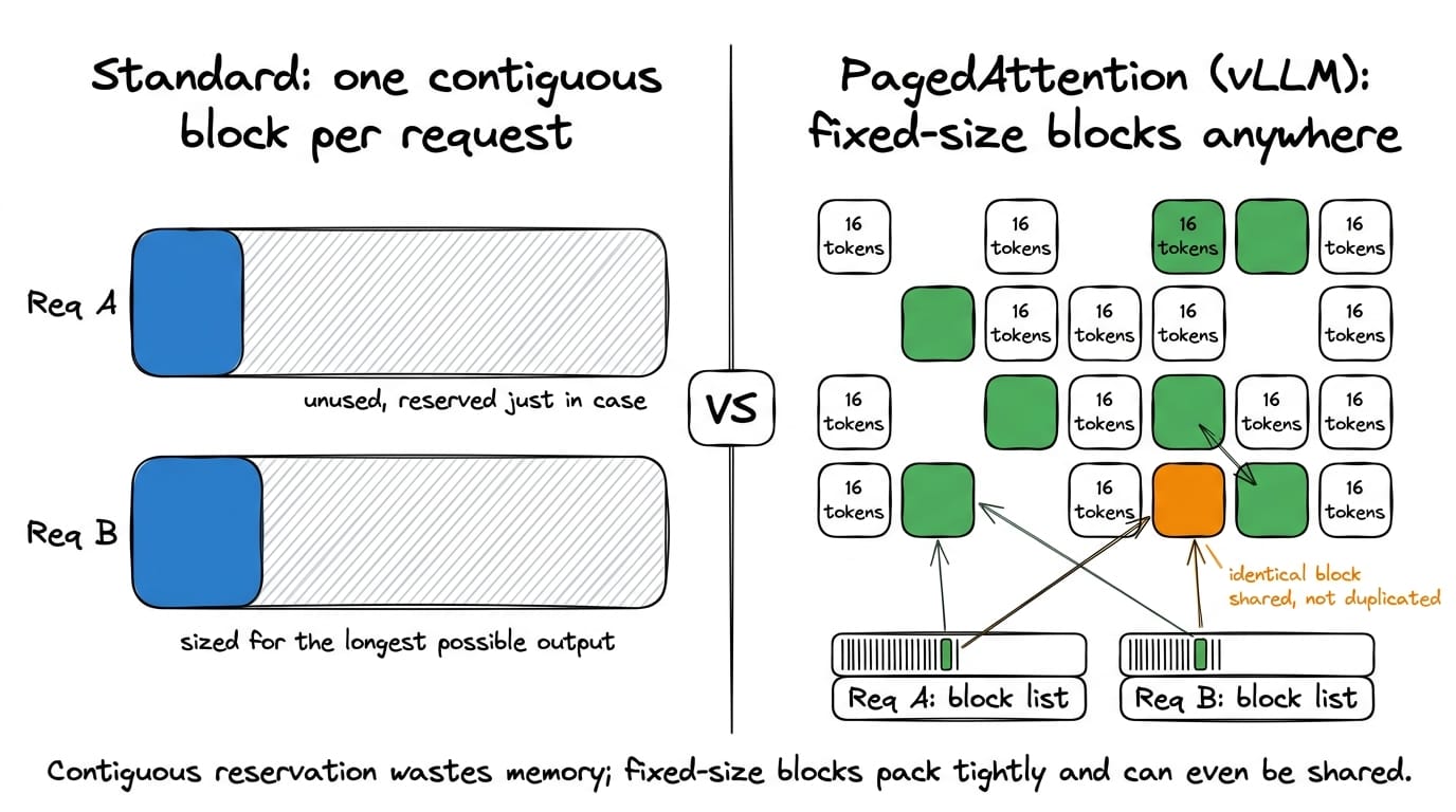
A typical block holds 16 tokens. The exact size is configurable and matters later, so it is worth remembering.

This design was built for memory efficiency, but it also enabled something else. More specifically, if blocks are independent units, then identical blocks can be shared between requests instead of being duplicated.

The hashing rule

Sharing blocks requires knowing when two blocks are genuinely identical. Automatic prefix caching solves this by hashing.

Each block is hashed together with the hash of every block before it. The stored key for a block is therefore not a function of its own tokens alone. It is a function of its tokens and its entire preceding context.

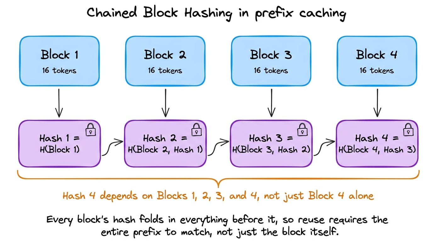
This rule is deliberate, and the reason for it is correctness.

A token's keys and values depend on everything the model saw before that token. Reusing a block only when the full prefix matches guarantees the reused values are bit-identical to what a fresh computation would produce.

So, a new request that begins with the same tokens as a cached request skips prefill for the shared portion. A long shared system prompt across many requests is the ideal case, and prefix caching handles it well.

The question is what happens when the shared content is not at the start.

Why prefix caching barely helps RAG

A RAG prompt is not one shared prefix followed by a short question. It is a system instruction, then several retrieved chunks, then the query. The chunks change per request, and their order changes too.

Watch what the hashing rule we discussed above does to that.

Suppose a request retrieves chunks $D_1$, $D_2$, and $D_3$, and the system caches all of them. A second request retrieves $D_1$, $D_2$, and $D_5$.

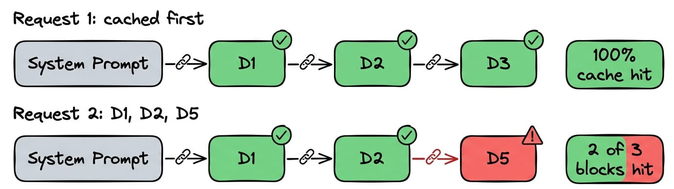
The first two chunks match, so their blocks are reused. The third does not, so it is recomputed. Two-thirds of the retrieved content is reused, which sounds acceptable.