A Crash Course on Building RAG Systems – Part 5 (With Implementation)

Introduction

If you’ve been following this RAG series, you’ve seen how we’ve steadily built up from the basics to advanced techniques, with each part laying the groundwork for the next.

RAG Crash Course - Daily Dose of Data Science

Daily Dose of Data ScienceAvi Chawla

Here’s a quick recap of what we’ve covered so far:

• In Part 1, we introduced the foundational components of RAG systems, exploring how text-based RAG systems are constructed and their key components.
• In Part 2, we focused on evaluation, diving into the metrics and methodologies to measure the accuracy, relevance, and reliability of RAG systems.
• In Part 3, we tackled the critical challenge of latency, discussing how to optimize text-based RAG systems for speed and efficiency, without compromising on accuracy.
• In Part 4, we expanded the scope beyond text to multimodal RAG systems, exploring how to parse, summarize, and store diverse data types like text, tables, and images.

Now, as we prepare to actually build a fully-fledged multimodal RAG system, there are a few critical techniques to cover first.

More specifically, to handle the intricacies of images, text, and structured data seamlessly, we need to explore three essential building blocks of a multimodal RAG system:

1) CLIP embeddings:

• These embeddings allow us to bridge the gap between images and text for efficient cross-modal understanding.
• We'll explore how CLIP (Contrastive Language-Image Pretraining) works and why it’s pivotal for multimodal RAG systems.

2) Multimodal prompting:

• Beyond standard text-based prompting, multimodal prompting enables RAG systems to process and reason about inputs that combine text, images, and more. These texts and images are supplied directly in the prompt, as shown below in the ChatGPT interface.

• So, in this section, we shall dive into the specifics of multimodal prompting and how it's done in a typical RAG system.

3) Tool calling:

• A strategy for enhancing the capabilities of RAG systems by dynamically calling external tools or APIs (e.g., OCR tools, table processors, or specialized ML models) when required.

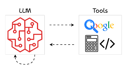
• Thus, in this section, we shall learn how these capabilities are enabled inside RAG systems.

Learning these techniques will set the stage for building practical multimodal RAG systems that can efficiently retrieve and process information across text, images, and structured data.

Let’s dive in!

1) CLIP embeddings

CLIP (Contrastive Language–Image Pretraining) is a model developed by OpenAI that creates a shared representation space for text and images.

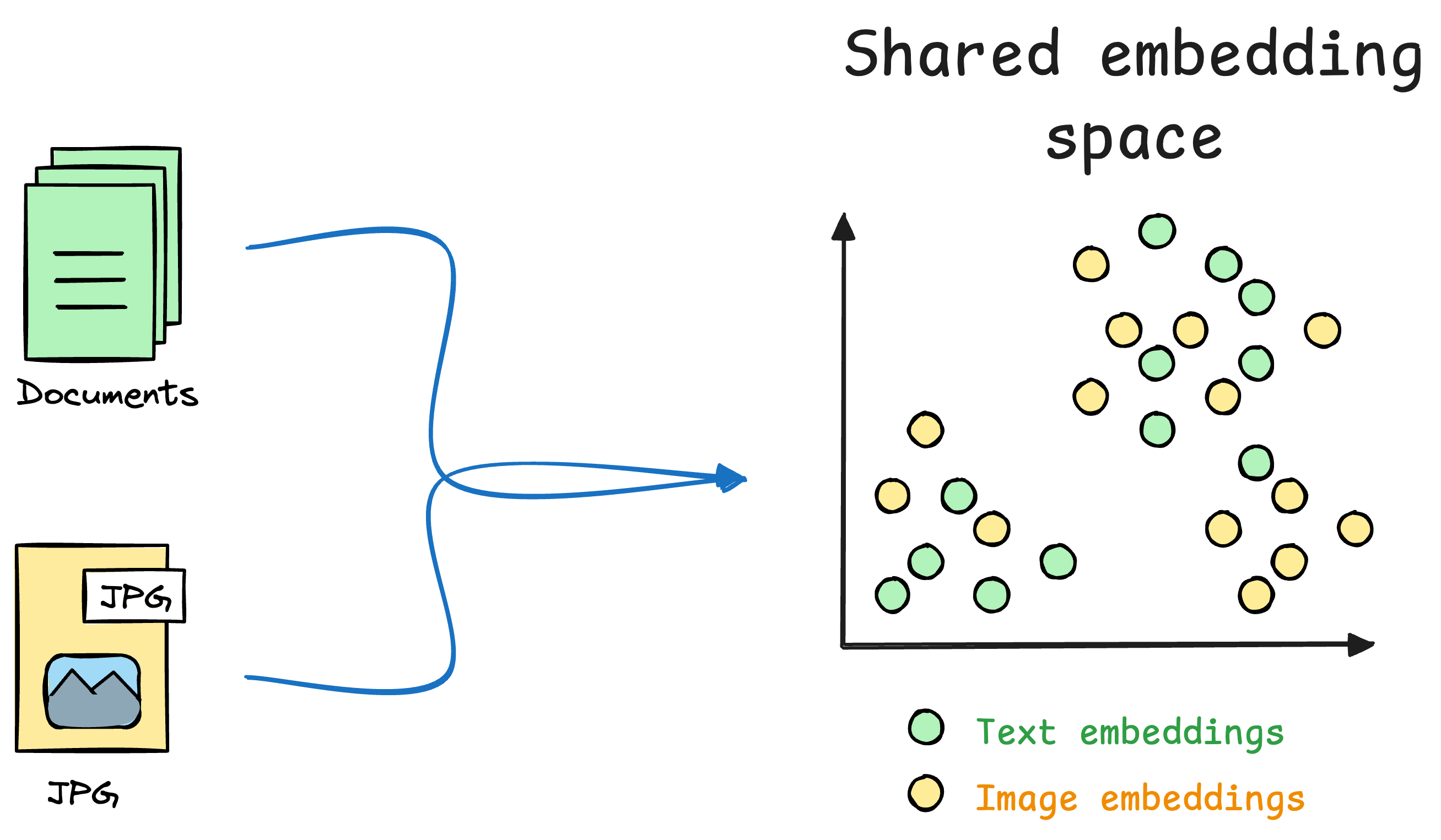
Unlike traditional models that handle text or images in isolation, CLIP allows us to compare and reason about text and images together, which makes it a key component of multimodal systems like Retrieval-Augmented Generation (RAG).

A key element of this model is Contrastive learning (which is also reflected in its name), so let's understand how Contrastive learning works below with a general use case.

Motivating task

As an ML engineer, you are responsible for building a face unlock system.

Let’s look through some possible options:

Option 1) How about a simple binary classification model?

Output 1 if the true user is opening the mobile; 0 otherwise.

Initially, you can ask the user to input facial data to train the model.

But that’s where you identify the problem.

All samples will belong to “Class 1.”

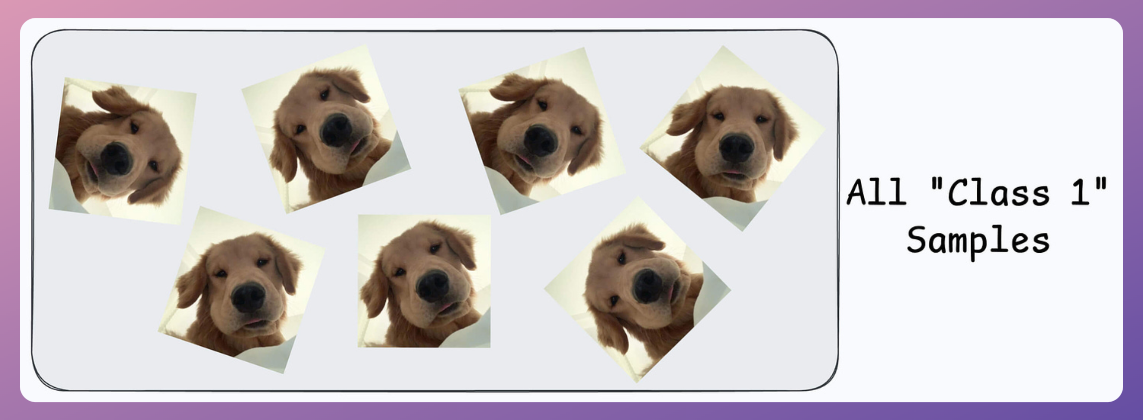
Now, you can’t ask the user to find someone to volunteer for “Class 0” samples since it’s too much hassle for them.

Not only that, you also need diverse “Class 0” samples. Samples from just one or two faces might not be sufficient.

The next possible solution you think of is…

Maybe ship some negative samples (Class 0) to the device to train the model.

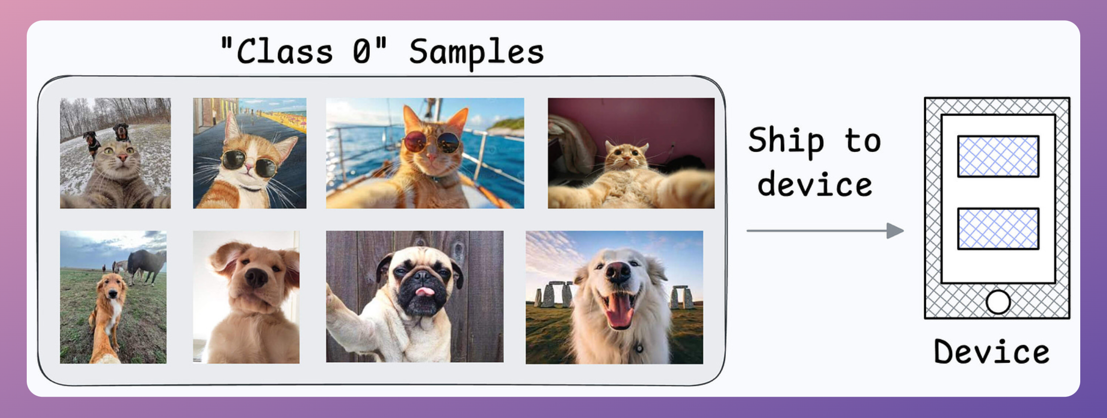
Might work.

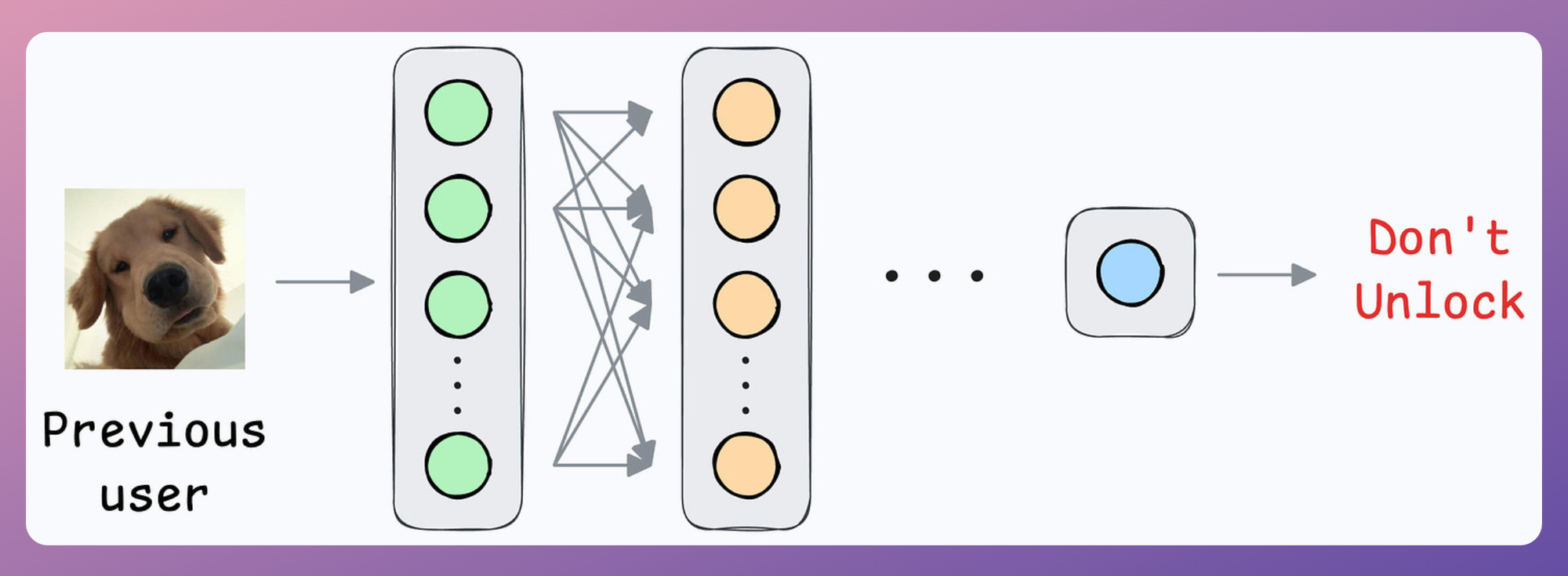
But then you realize another problem:

What if another person wants to use the same device?

Since all new samples will belong to the “new face” during adaptation, what if the model forgets the first face?

Option 2) How about transfer learning?

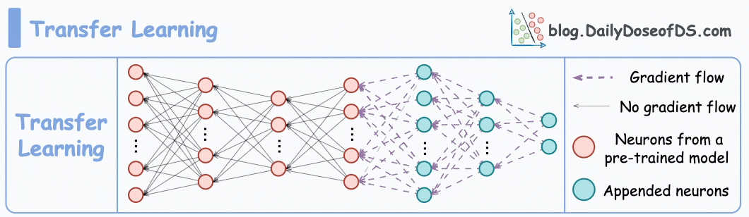
This is extremely useful when:

• The task of interest has less data.
• But a related task has abundant data.

This is how you think it could work in this case:

• Train a neural network model (base model) on some related task → This will happen before shipping the model to the user’s device.
• Next, replace the last few layers of the base model with untrained layers and ship it to the device.

It is expected that the first few layers would have learned to identify the key facial features.

From there on, training on the user’s face won’t require much data.

But yet again, you realize that you shall run into the same problems you observed with the binary classification model since the new layers will still be designed around predicting 1 or 0.

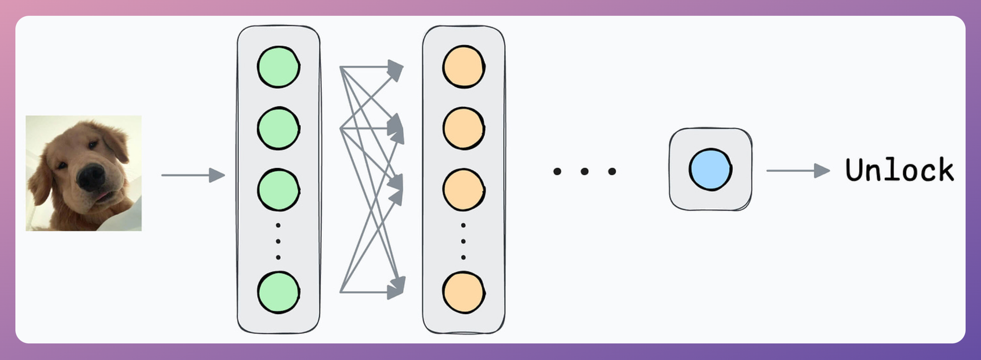
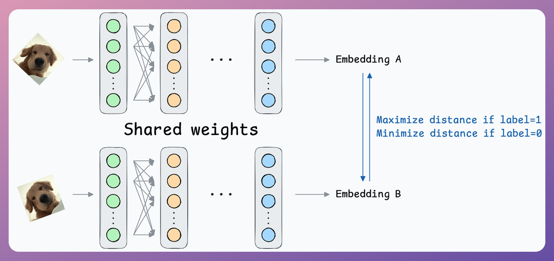
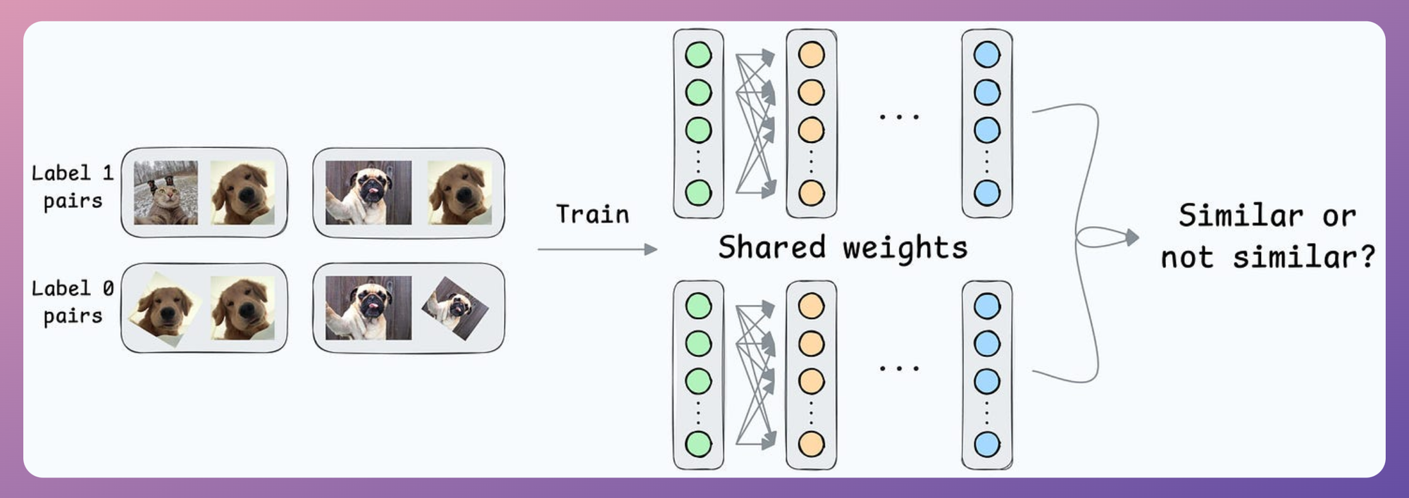
Solution: Contrastive learning using Siamese Networks

At its core, a Siamese network determines whether two inputs are similar.

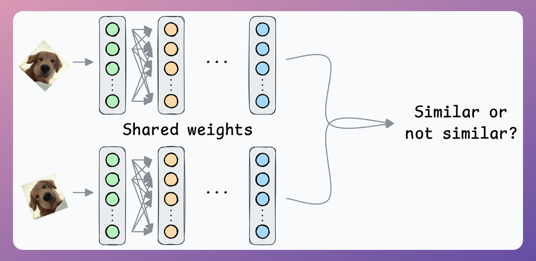
It does this by learning to map both inputs to a shared embedding space (the blue layer above):

• If the distance between the embeddings is LOW, they are similar.
• If the distance between the embeddings is HIGH, they are dissimilar.

They are beneficial for tasks where the goal is to compare two data points rather than to classify them into predefined categories/classes.

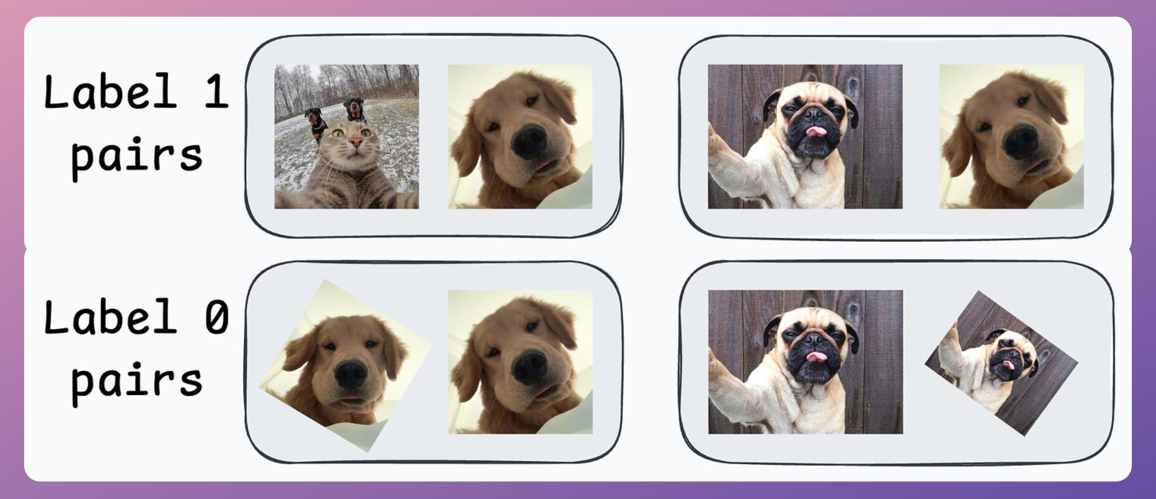
This is how it will work in our case:

• If a pair belongs to the same person, the true label will be 0.
• If a pair belongs to different people, the true label will be 1.

Create a dataset of face pairs:

Pass both inputs through the same network to generate two embeddings.

• If the true label is 0 (same person) → minimize the distance between the two embeddings.
• If the true label is 1 (different person) → maximize the distance between the two embeddings.

After creating this data, define a network like this:

Contrastive loss (defined below) helps us train such a model:

where:

• y is the true label.
• D is the distance between two embeddings.
• margin is a hyperparameter, typically greater than 1.

Here’s how this particular loss function helps:

When y=0 (same person), the loss will be:

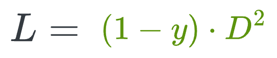
• The above value will be minimum when D is close to 0, leading to a low distance between the embeddings.

When y=1 (different people), the loss will be:

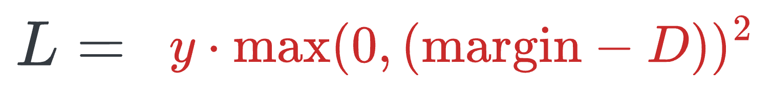
• The above value will be minimum when D>margin, leading to more distance between the embeddings.

This way, we can ensure that:

• when the inputs are similar, they lie closer in the embedding space.
• when the inputs are dissimilar, they lie far in the embedding space.

Siamese Networks in face unlock

Here’s how it will help in the face unlock application.

First, you will train the model on several image pairs using contrastive loss.

This model (likely after model compression) will be shipped to the user’s device.

During the setup phase, the user will provide facial data, which will create a user embedding:

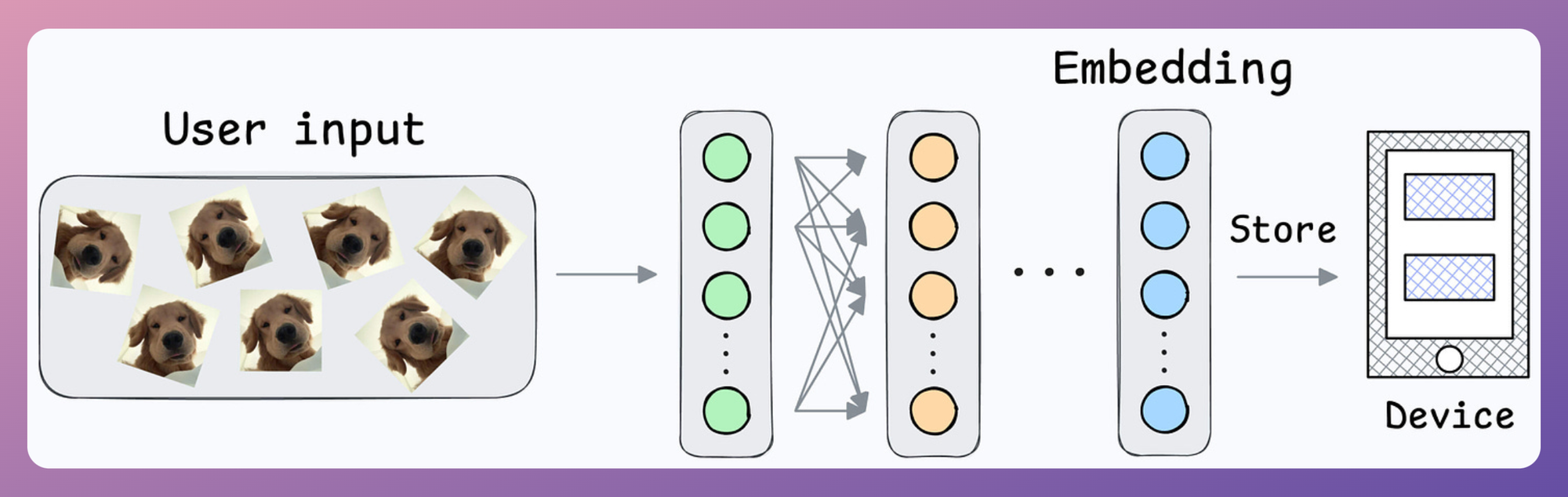
This embedding will be stored in the device’s memory.

Next, when the user wants to unlock the mobile, a new embedding can be generated and compared against the available embedding:

• Action: Unlock the mobile if the distance is small.

Done!

Note that no further training was required here, like in the earlier case of binary classification.

Also, what if multiple people want to add their face IDs?

No problem.

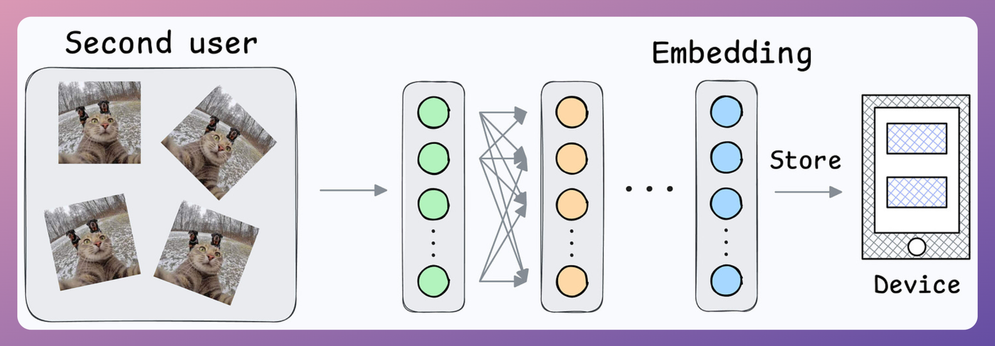
We can create another embedding for the new user.

During unlock, we can compare the incoming user against all stored embeddings.

Implementing Contrastive Learning-based Siamese Network

Next, let’s look at the implementation of this model.

For simplicity, we shall begin with a simple implementation utilizing the MNIST dataset. In a future issue, we shall explore the face unlock model.

Let’s implement it.

As always, we start with some standard imports:

Next, we download/load the MNIST dataset:

Now, recall to build a Siamese network, we have to create image pairs:

• In some pairs, the two images will have the same true label.
• In other pairs, the two images will have a different true label.

To do this, we define a SiameseDataset class that inherits from the Dataset class of PyTorch:

This class will have three methods:

• The __init__ method:

In the above code, the data parameter will be mnist_train and mnist_test defined earlier.

• The __len__ method:

• The __getitem__ method, which is used to return an instance of the train data. In our case, we shall pair the current instance from the training dataset with:
  • Either another image from the same class as the current instance.
  • Or another image from a different class.
  • Which class to pair with will be decided randomly.

The __getitem__ method is implemented below:

• Line 5: We obtain the current instance.
• Line 7: We randomly decide whether this instance should be paired with the same class or not.
• Lines 9-12: If flag=1, continue to find an instance until we get an instance of the same class.
• Lines 14-17: If flag=0, continue to find an instance until we get an instance of a different class.
• Line 19-21: Apply transform if needed.
• Line 23:
  • If the two labels are different, the true label for the pair will be 1.
  • If the two labels are the same, the true label for the pair will be 0.

After defining the class, we create the dataset objects below:

Next, we define the neural network:

As demonstrated in the above code, the two input images are fed through the same network to generate an embedding (outputA and outputB).

Moving on, we define the contrastive loss:

Almost done!

Next, we define the dataloader, the model, the optimizer, and the loss function:

Finally, we train it:

And with that, we have successfully implemented a Siamese Network using PyTorch.

Results

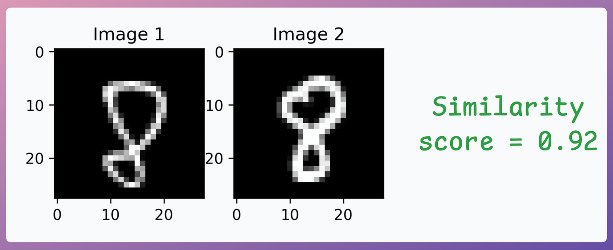
Let’s look at some results using images in the test dataset:

We can generate a similarity score as follows:

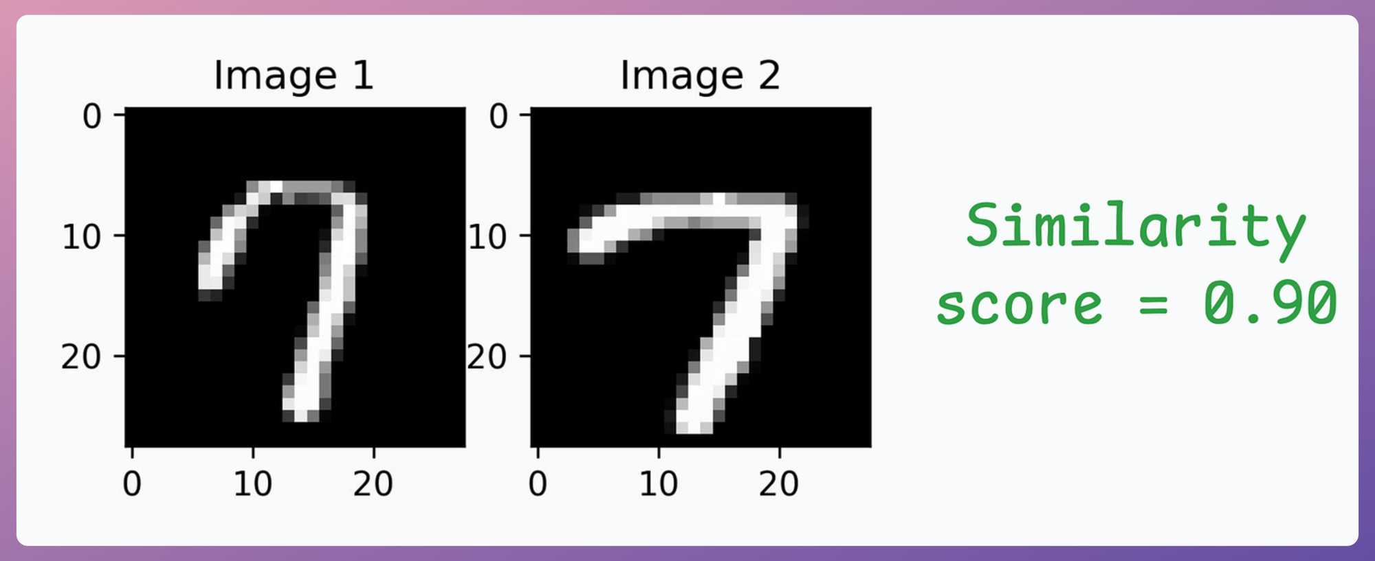
• Image pair #1: Similarity is high since both images depict the same digit:

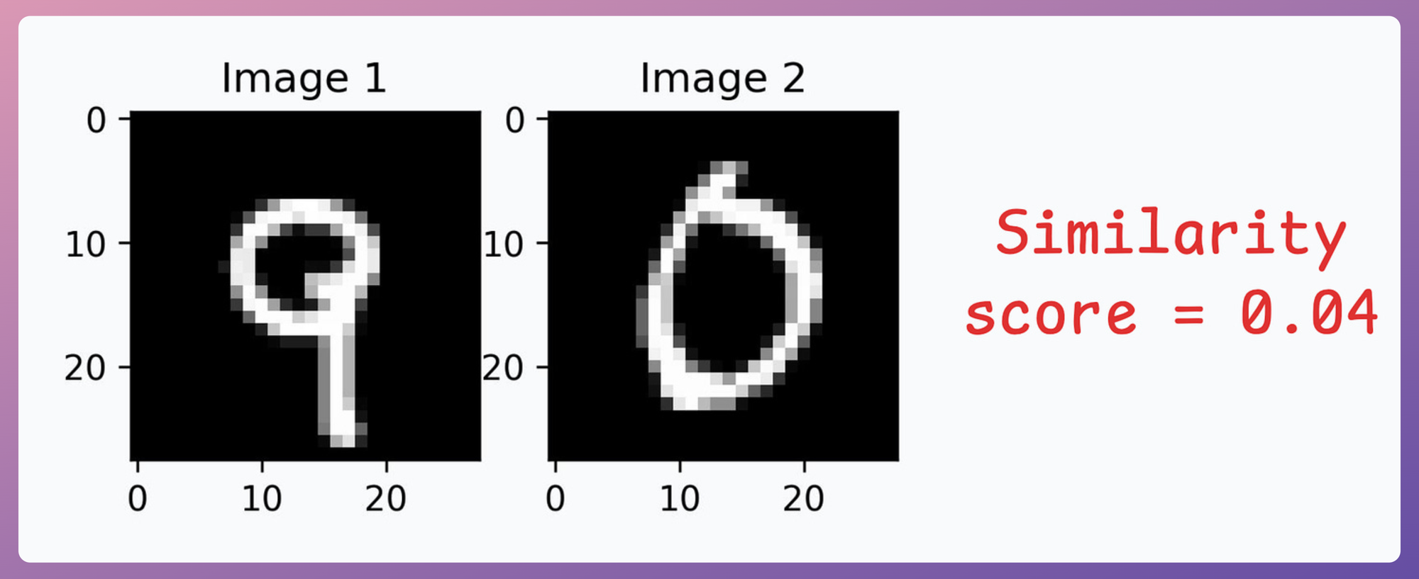
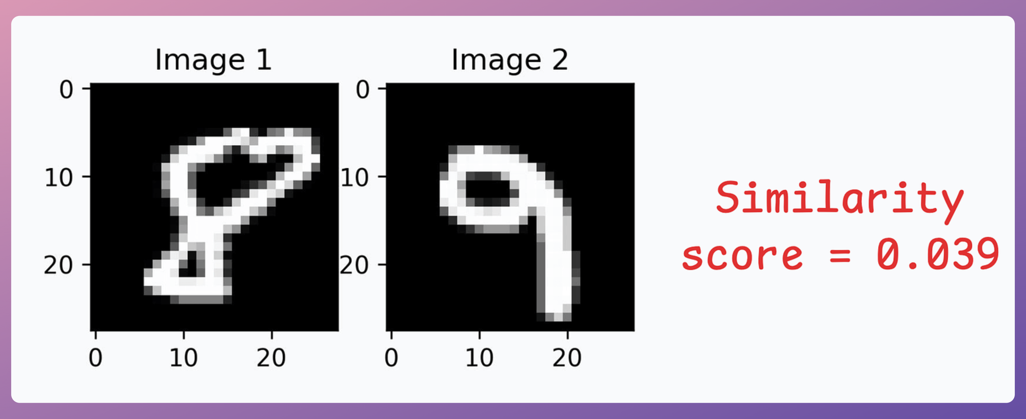
• Image pair #2: Similarity is low since both images depict different digits:

• Image pair #3: Similarity is high since both images depict the same digit:

• Image pair #4: Similarity is low since both images depict different digits:

Great, it works as expected!

This is the whole idea behind contrastive learning, which is also leveraged in CLIP.

In the above discussion about face unlock systems, a shared encoder network was used to embed both inputs (e.g., pairs of images) into the same vector space. The similarity or dissimilarity between the inputs was determined by their distance in this space, guided by a contrastive loss.

However, CLIP takes this a step further by employing two distinct encoders:

• One for text and
• Another for images.

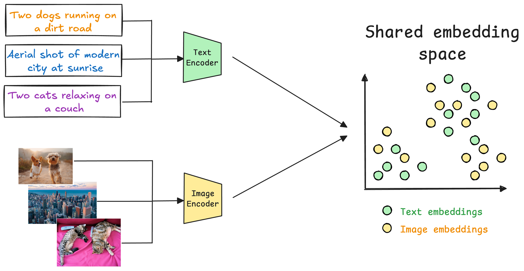
These encoders map their respective modalities (text and image) into a shared multimodal embedding space. This enables a cross-modal comparison—a text can be compared to an image, or vice versa, to evaluate their semantic similarity, which is a key component of a multimodal RAG system.

CLIP model training

Just like the above MNIST implementation, once you have gathered a text-image pair dataset, the next step is training the CLIP model through contrastive learning, which pushes embeddings of related pairs closer together while pulling embeddings of unrelated pairs further apart.

Here’s how the process works:

1) Preparing the dataset

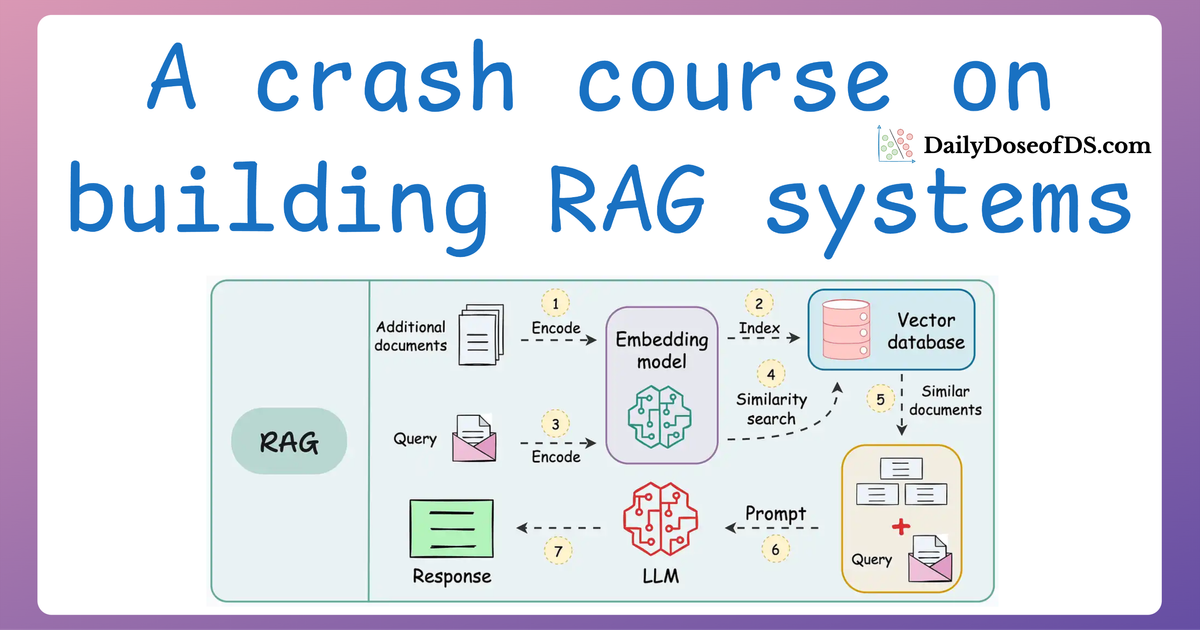
A text-image pair dataset is required, where each pair consists of:

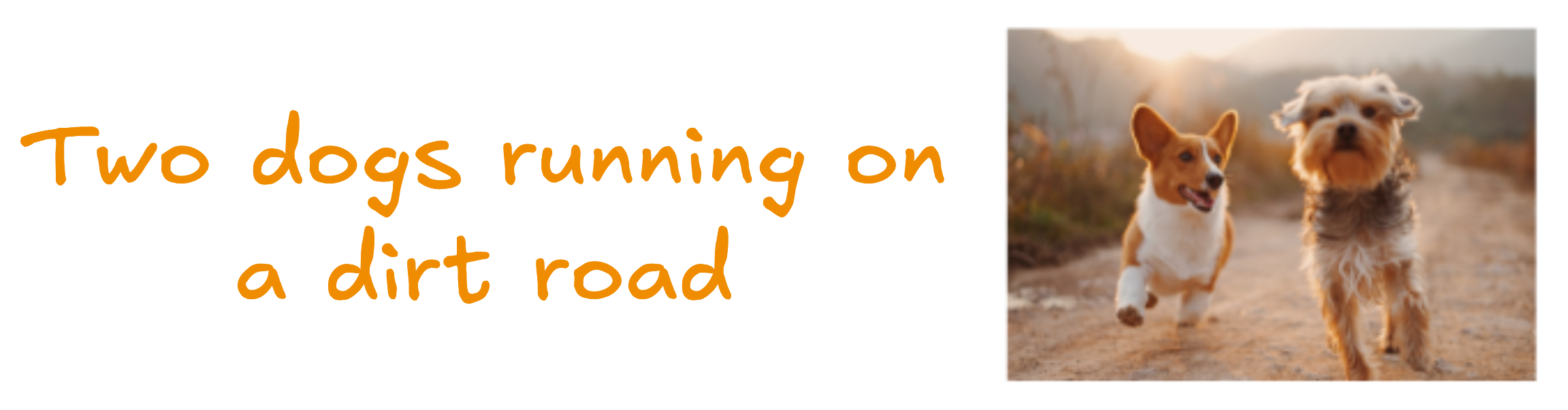
• A text description (e.g., "Two dogs running on a dirty road")
• Its corresponding image (e.g., an image of two dogs running on a dirty road).

These pairs are treated as positive samples (related). Negative samples are implicitly generated by pairing unrelated text and images from the dataset.

2) Passing inputs through the encoders

The text encoder processes the text descriptions to generate text embeddings, and the image Encoder processes the images to generate image embeddings.

3) Contrastive Learning with cross-modal similarity

To align text and image embeddings, a contrastive loss function is applied. The goal is:

• To maximize the similarity between embeddings of matched (text, image) pairs.
• To minimize similarity between embeddings of mismatched (text, image) pairs.

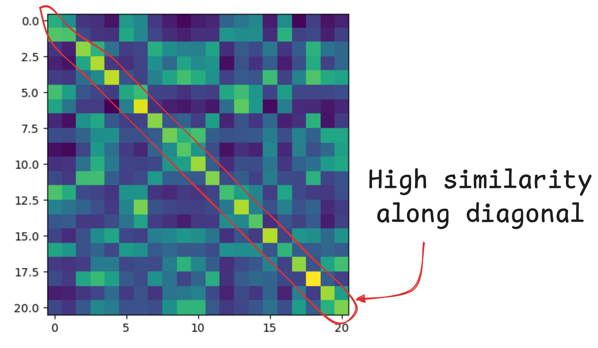
For instance, in the image above, all pairs along the diagonal contribute to positive examples, and all other pairs contribute to negative examples.

Finally, the network is trained using the contrastive loss function we discussed earlier.

• For each positive pair, the loss encourages a low distance (close to 0) between embeddings.
• For each negative pair, the loss encourages a high distance between embeddings.

And this is how we build a CLIP model.

CLIP demo

Now that we understand the foundational details of building a multimodal LLM, let's look at a demo of the pre-trained CLIP model and how we can use it for:

• Text-to-image search
• Image-to-image search
• Zero-shot classification

Setup

First, start with some installations:

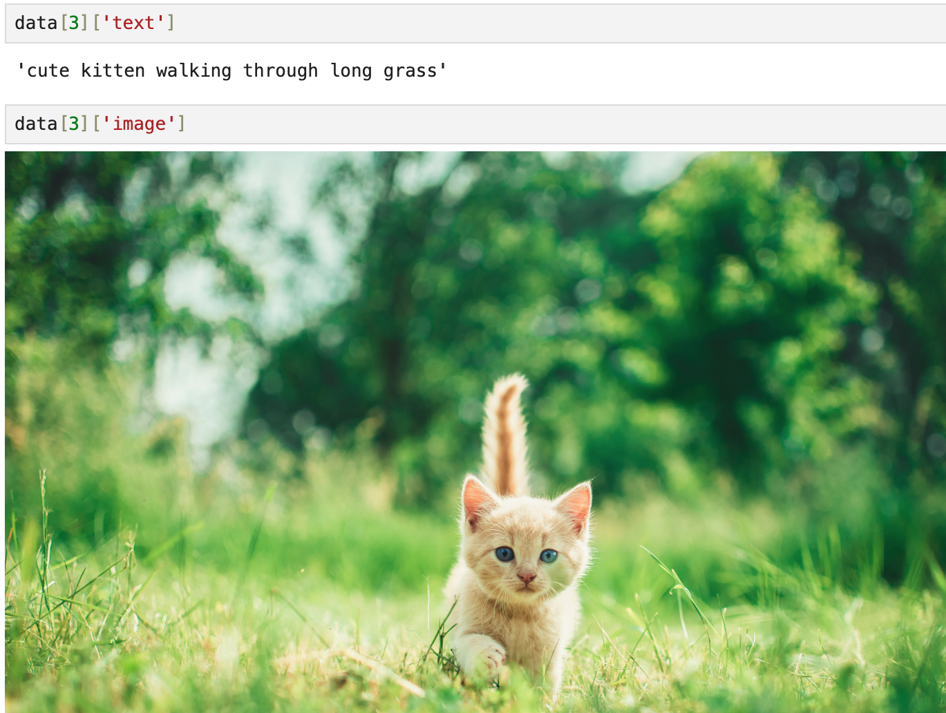
Next, we are going to use this dataset, which provides several image text pairs:

jamescalam/image-text-demo · Datasets at Hugging Face

We’re on a journey to advance and democratize artificial intelligence through open source and open science.

Download and load it using the datasets library as follows:

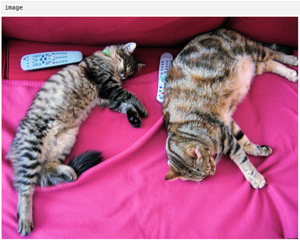
We can directly preview an image-text pair as follows:

Now, let's set up the CLIP model using Hugging Face's transformers library. In this example, we'll use OpenAI’s pre-trained clip-vit-base-patch32 model, a popular and lightweight version of CLIP.

This is demonstrated below:

As depicted above, we use the standard procedures of using models from Huggingface by importing the necessary components—CLIPProcessor for preprocessing and CLIPModel for loading the CLIP architecture. The model and processor are both loaded using the from_pretrained method.

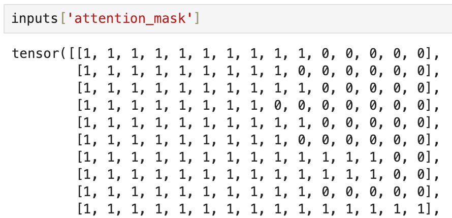
The next step involves preparing inputs for CLIP by using the processor defined earlier to handle both text and image data seamlessly.

Here, text and images are extracted from the dataset. These inputs are passed to the processor with the following arguments:

• text=text: Specifies the text descriptions, which will be tokenized and converted into the format expected by the text encoder.
• images=images: Specifies the batch of images, which will be padded/resized to meet the image encoder's input requirements.
• return_tensors="pt": Ensures that the outputs are returned as PyTorch tensors, compatible with the CLIP model.
• padding=True: Adds padding to text sequences to ensure they have consistent lengths within the batch.

The resulting inputs object contains the preprocessed data for both the text and image encoders, and it includes:

• input_ids: Tokenized representations of the text inputs.
• attention_mask: Attention masks for the text inputs, where 0 denotes the padding token:

• pixel_values: Preprocessed image tensors.

The next step is to pass them through the CLIP model to obtain the outputs, as demonstrated below:

In the above code, the inputs dictionary (containing both text and image tensors) is unpacked and fed into the model. The model processes the data through its dual encoders:

• The text encoder generates embeddings for the tokenized text inputs.
• The image encoder generates embeddings for the preprocessed image inputs.

The resulting outputs object contains the embeddings and additional information, which you can explore by calling outputs.keys().

The output keys that are of relevance to us are text_embeds and image_embeds:

Going back to our earlier discussion, it is expected that if we measure the similarity between the above two embedding matrices, all pairs along the diagonal of that similarity matrix will indicate positive examples, and all other pairs will indicate negative examples.

Let's measure this below:

Next, let's plot this as a heatmap:

This produces the following plot, which depicts high similarity along the diagonal:

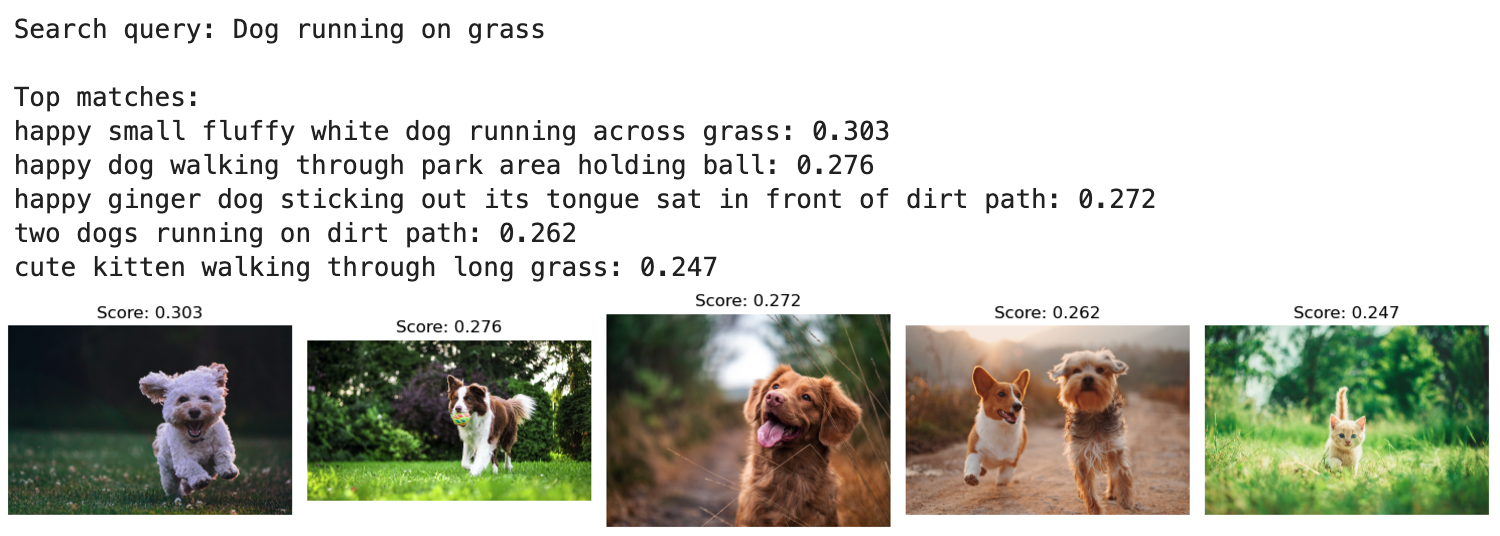
Text-to-image search

Since every image and text has a corresponding embedding in a shared embedding space, we can use those embeddings for retrieval.

Let's say I have a text prompt. I can embed it using my text encoder in the CLIP model, match it across the embeddings of all images in the vector database, and then fetch the top results.

Logically, it's quite easy to implement, as demonstrated in the code below:

• The text query is tokenized and converted into PyTorch tensors using the processor.
• The preprocessed input is then passed through the model's text encoder to generate the text embedding (text_features).
• The embedding is then normalized before calculating similarity scores.
• Next, the similarity between the text embedding and all image embeddings is calculated.
• Finally, using PyTorch's topk function, the top-k images with the highest similarity scores are retrieved.

We can display these results as follows:

This produces the following top-5 matches, which mostly look great.

Wasn't that simple?

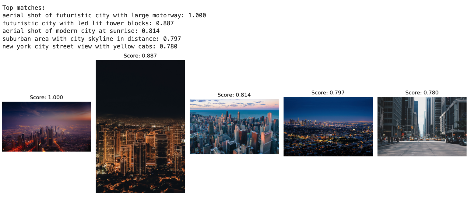
Image-to-image search

A large part of building multimodal RAG apps also involves image-to-image similarities, so next, let's look at how we can do an image-to-image search using CLIP.

The logical steps will remain the same as before:

• The image is preprocessed using the processor.
• The preprocessed input is then passed through the model's image encoder to generate the image embedding (image_features).
• The embedding is then normalized before calculating similarity scores.
• Next, the similarity between the image embedding and all other image embeddings is calculated.
• Finally, using PyTorch's topk function, the top-k images with the highest similarity scores are retrieved.

The query image input, in this case, is the following image:

We can display the retrieved results as follows:

This produces the following top-5 matches, which mostly look great.

Zero-shot classification

Zero-shot classification is a paradigm in machine learning where a model can classify data into categories it has never explicitly been trained on.

Since the model has already been trained on vast amounts of datasets, it does not require any further labeled examples for each class. Instead, the model can leverage semantic understanding to generalize to new, unseen classes using natural language descriptions.

Here's a quick demo of using CLIP for zero-shot classification:

• First, we gather an image that's available online:

• We have the following image:

• Next, we preprocess it and pass it through the model:

• Now, here's something to note about this code.
• Since this is a classification task, we would already know the classes that we want to classify our new data into.
• Thus, in the text argument, instead of passing "dog" and "cat", we pass the descriptions of our class so that the semantic similarity between text and image remains coherent with how the model was originally trained.
• That said, once we have obtained the output, we can obtain the logits and generate the corresponding softmax scores as follows:

The softmax scores show high similarity with the description “a photo of a cat”, which is indeed correct.

2) Multimodal prompting

As the name suggests, multimodal prompting extends the concept of natural language prompting to include multiple data modalities, such as text, images, videos, and structured data.

In traditional text-only prompting (early versions of ChatGPT, for instance), users provide textual instructions or queries to guide the behavior of a model.

Multimodal prompting builds on this by allowing prompts that combine text with other modalities, such as:

• Images: Provide visual context or ask questions about visual content.
• Tables: Supply structured data for reasoning.
• Audio or Video: Enable dynamic, context-aware queries based on audio-visual inputs.

Prerequisites and installations

Since we have always used Ollama in our previous parts, we will stick with it and learn about multimodal prompting.

Ollama provides a platform to run LLMs locally, giving you control over your data and model usage.

Here's a step-by-step guide on using Ollama.

• Go to Ollama.com, select your operating system, and follow the instructions.

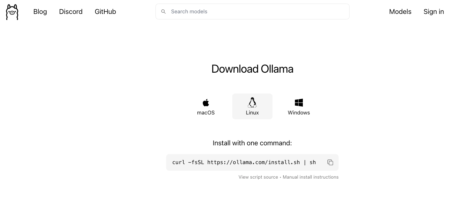
• If you are using Linux, you can run the following command:

• Ollama supports a bunch of models that are also listed in the model library:

library

Get up and running with large language models.

Once you've found the model you're looking for, run this command in your terminal:

The above command will download the model locally, so give it some time to complete. But once it's done, you'll have Llama 3.2 3B running locally, as shown below, which depicts Microsoft's Phi-3 served locally through Ollama:

For this article, we shall pull the Llama3.2-vision model as follows:

Also, install the Ollama Python package as follows:

Done!

The standard way to prompt a model with Ollama is as follows (here, we are not using images):

• The model parameter specifies the model you want to use (must be available locally).
• The messages parameter specifies the interaction history with the LLM.

This produces the following output, which says the author is J.R.R. Tolkien:

Let's understand the format for interaction history in a bit more detail since it's going to be useful for us to build interaction-driven apps.

Supported roles

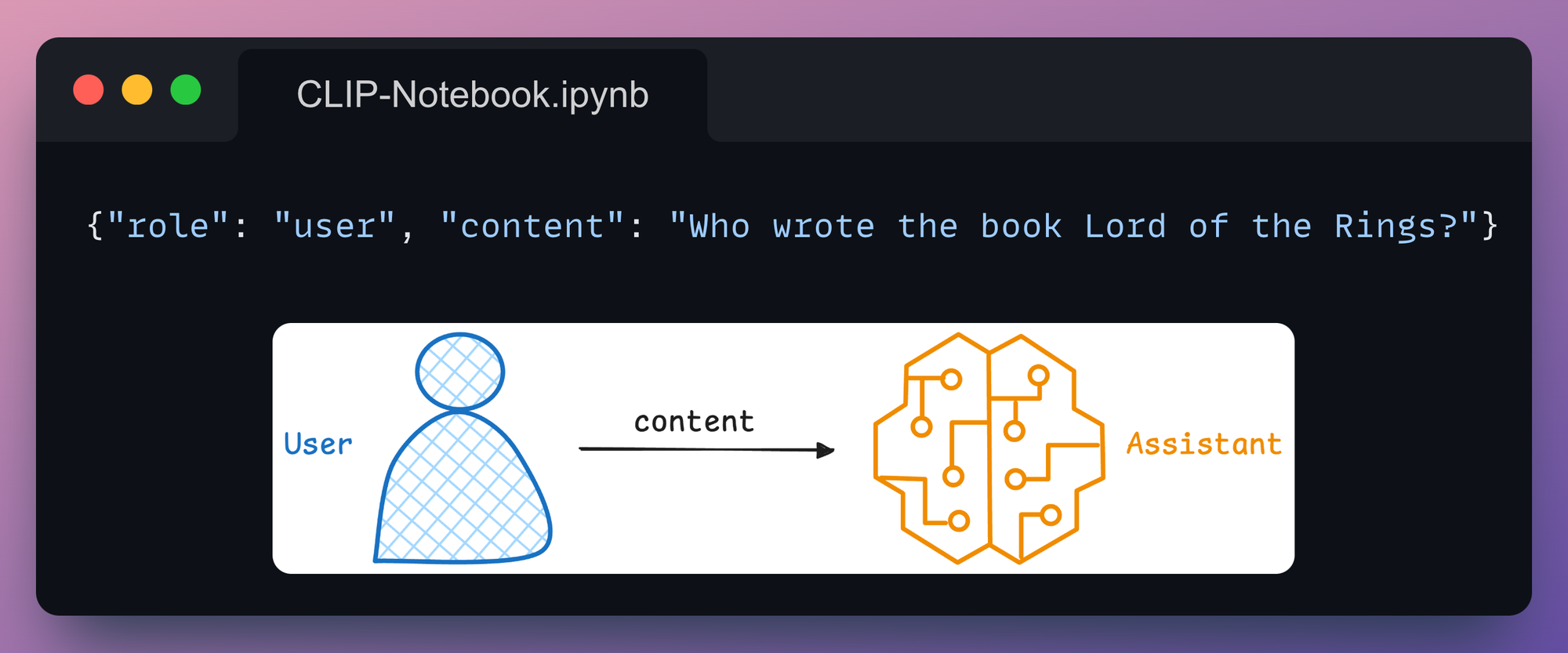
Here, messages represent the structured inputs used to define the interaction. These messages often include a role and content to specify the nature of the interaction and the information being exchanged.

There are three roles in such systems:

1) User

This represents the input or query provided by the user interacting with the system.

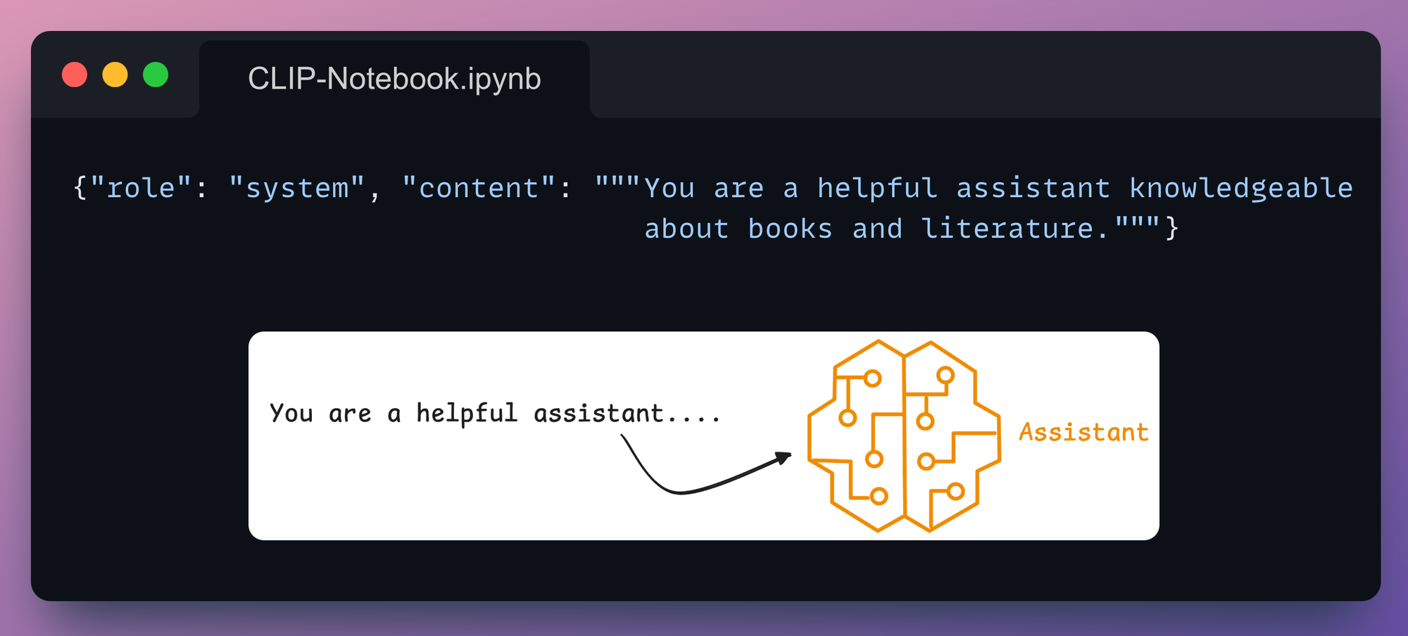
2) System

This sets the behavior or persona of the AI model. This role is often used to prime the model for specific tasks or tones.

3) Assistant

This represents the AI's response to the user query based on the system's instructions and user inputs.

All these three roles, when used together, define a structured dialogue and let the model have access to the full context and history when it's responding to new queries.

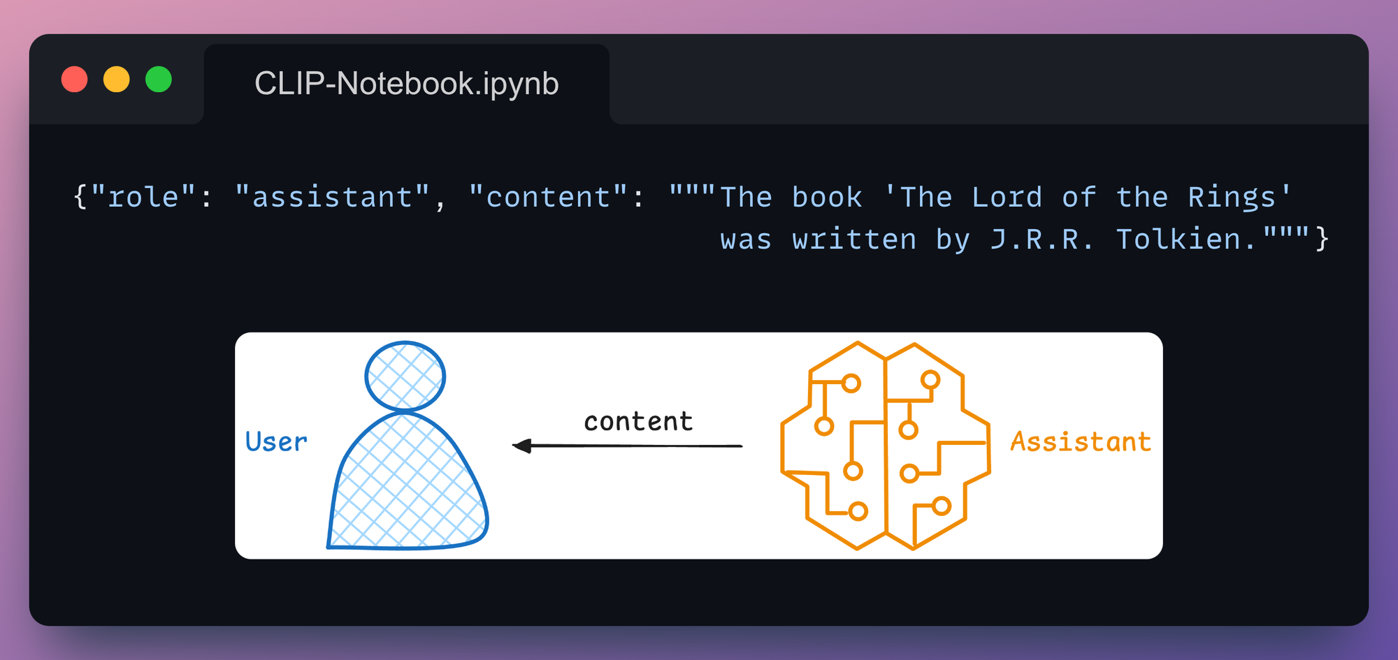
For instance, let's go back to our initial prompt:

In the above code, the model's output was stored in response1. Let's ask a follow-up question on this by appending this response to the messages parameter.

This is implemented below:

This time, we get the following output:

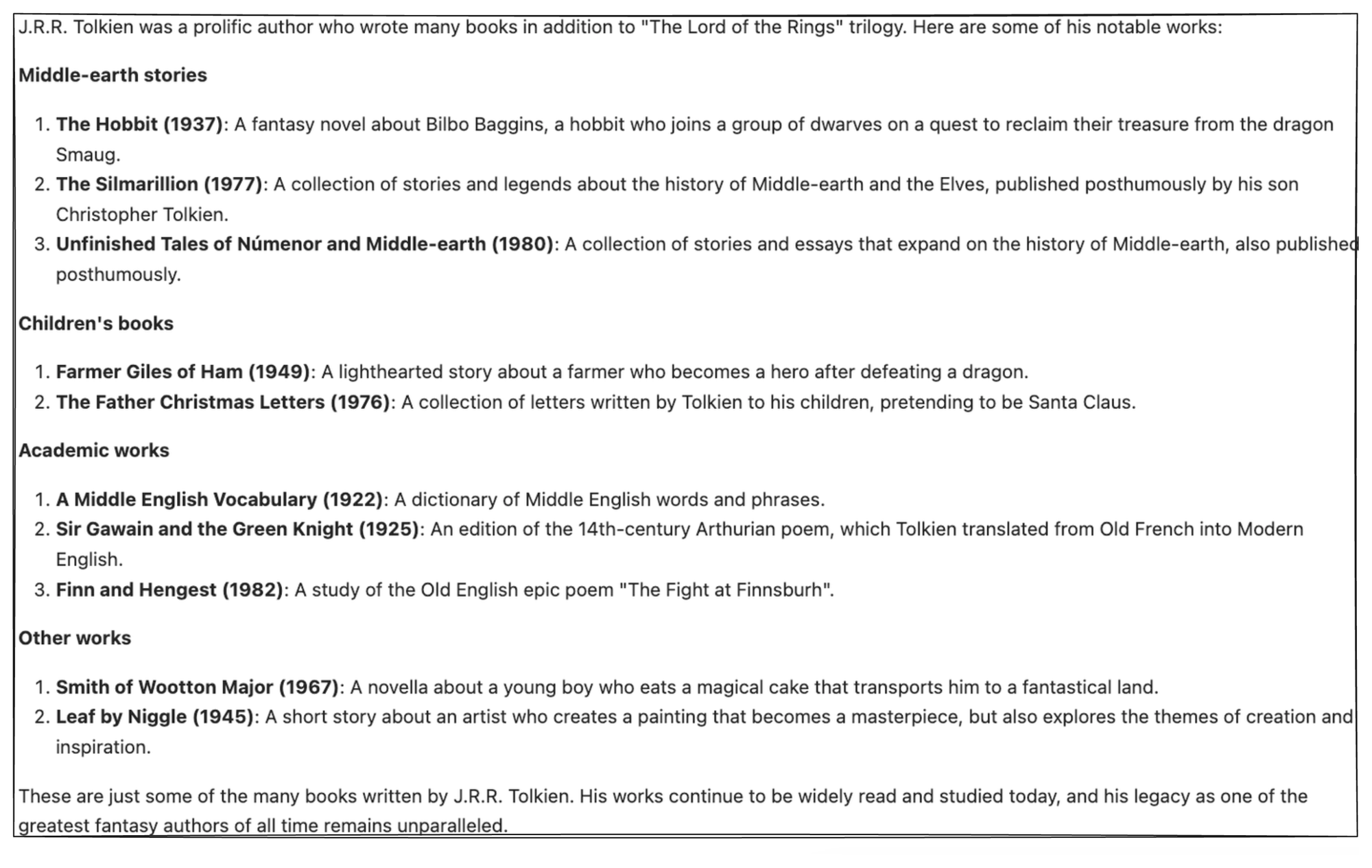
Notice that we never specified in the new query that we are asking about J.R.R. Tolkien. Yet, it was able to respond with the notable works of this works just because it had access to the context.

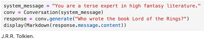
The above approach appears a bit messy, so let's organize what we've done so far by creating a Conversation class:

In the above code:

• When an instance of Conversation is created, an optional system message can be provided to set the behavior or persona of the AI (e.g., "You are a helpful assistant knowledgeable about movies.").
• The generate method handles the user’s query and generates a response from the LLM:
  • The user_question is appended to the self.messages list with the "user" role.
  • The ollama.chat function interacts with the AI model (e.g., llama3.2-vision) using the current conversation history (self.messages) as input.
  • The model's response is appended to the self.messages list with the "assistant" role.

Next, we can instantiate this class and launch a chat:

This produces the following response:

Displaying the messages attribute, we get:

Specify images in prompts

If the above discussion is clear, extending this to a multimodal input, like images + text, is quite simple with Ollama.

Consider you have this image stored in your local directory (download below):

You can prompt the multimodal LLM with the image as follows:

If you have multiple images, you can pass them as a list in the images key of messages parameter.

A realistic OCR use case

You may have already seen us talk about this.

Recently, we created our own OCR app using the Llama-3.2-vision model, which was built using multimodal prompting.

So let us show you how we did this.

In this app, you can upload an image, and it converts it into a structured markdown using the Llama-3.2 multimodal model, as shown in this demo:

The entire code is available here: ​Llama OCR Demo GitHub.

In this case, we can prompt Llama3.2-vision with Ollama as follows:

Done!

Of course, the full Streamlit app will require more code to build, but everything is still just 50 lines of code, and this isn't the goal here.

Instead, the goal is to demonstrate how simple it is to use frameworks like Ollama to build LLM apps.

In the app we built, you can upload an image, and it converts it into a structured markdown using the Llama-3.2 multimodal model, as shown in this demo:

With that, we conclude multimodal prompting.

Let's move to the final section of tool calling.

3) Tool calling

As the name suggests, tool calling refers to the ability of AI models to invoke external tools or APIs to perform specific tasks beyond their built-in capabilities.

This is especially important since there can be several stages in the generation process where AI might need to process diverse data types, fetch live data, or perform specialized computations.

So, in a gist, this is what the process looks like:

1. Recognize when a task requires external assistance.
2. Invoke the appropriate tool or API for that task.
3. Process the tool's output and integrate it into its response.

This approach turns the AI into more like a coordinator, delegating tasks it cannot handle internally to specialized tools.

A recent newsletter issue where we talked about ReAct Agent is a classic example of this:

Intro to ReAct (Reasoning and Action) Agents

...and building one with Dynamiq.

Daily Dose of Data ScienceAvi Chawla

Demo

Assuming the motivation is clear, let's do a demo of Tool Calling.

We’ll build a simple stock price retrieval assistant that combines the natural language capabilities of Ollama’s Llama model with the real-time data retrieval capabilities of the yfinance library.

The AI will intelligently recognize when it needs to call a tool (in this case, a Python function for fetching stock prices) and integrate the results into its response.

Get started by installing yfinance:

Next, the tool function, get_stock_price, uses the yfinance library to fetch the latest closing price for a specified stock ticker:

• This function accepts the ticker, which is the stock ticker symbol (e.g., "AAPL" for Apple).
• It returns the latest closing price of the stock.

Next, using Ollama’s Llama model, the assistant identifies queries requiring the use of external tools and generates tool calls as part of its response. The tools are passed to the model as a list:

• The messages parameter defines the conversation context.
• The tools parameter provides a reference to the available external tools.

If we print the response object, we get this output:

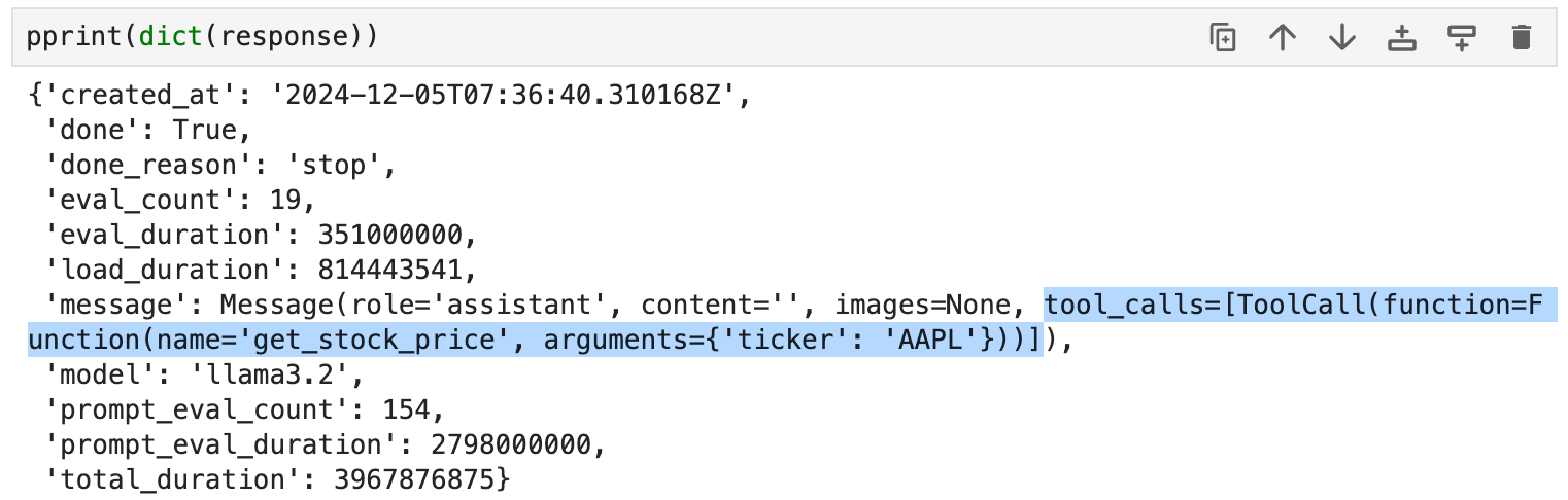
Notice that the message key in the above response object includes tool_calls along with the argument.

And this tool_calls attribute contains the relevant details, such as:

• tool.function.name: The name of the tool to be called.
• tool.function.arguments: The arguments required by the tool.

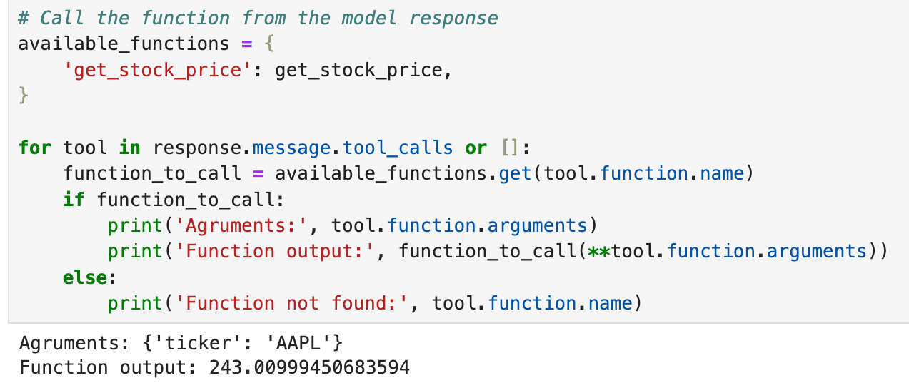
Thus, we can utilize this info to produce a response as follows:

• We iterate over all the functions in the tool_calls attribute.
• We get the function object and invoke it.

Done!

This produces the following output.

Of course, the above output can also be passed back to the AI to generate a more vivid response. We'll leave it to you as an exercise.

But one thing must be clear: with tool calling, the assistant can be made more flexible and powerful to handle diverse user needs.

Conclusion

With that, we come to the end of Part 5 of our RAG crash course.

In this article, we took a slight but necessary detour to cover some of the fundamental concepts necessary for understanding and implementing multimodal prompting.

We explored:

• CLIP embeddings, which help these systems align text and image data in a shared semantic space and enable cross-modal tasks like image-to-image search, text-to-image search and zero-shot classification.
• Multimodal prompting, which lets the user provide inputs that span multiple modalities.
• Tool calling, a mechanism to extend the model’s capabilities by dynamically invoking external tools or APIs to fetch real-time data or handle specialized tasks.

With that, we are set to build multimodal RAG systems.

So, in the upcoming part, we’ll put this knowledge into action and begin constructing our multimodal RAG system.

Thanks for reading!

Any questions?

Feel free to post them in the comments.

Or

If you wish to connect privately, feel free to initiate a chat here: