A Beginner-friendly and Comprehensive Deep Dive on Vector Databases

Introduction

It’s pretty likely that in the generative AI era (since the release of ChatGPT, to be more precise), you must have at least heard of the term “vector databases.”

It’s okay if you don’t know what they are, as this article is primarily intended to explain everything about vector databases in detail.

But given how popular they have become lately, I think it is crucial to be aware of what makes them so powerful that they gained so much popularity, and their practical utility not just in LLMs but in other applications as well.

Let’s dive in!

What are vector databases?

Objective

To begin, we must note that vector databases are NOT new.

In fact, they have existed for a pretty long time now. You have been indirectly interacting with them daily, even before they became widely popular lately. These include applications like recommendation systems, and search engines, for instance.

Simply put, a vector database stores unstructured data (text, images, audio, video, etc.) in the form of vector embeddings.

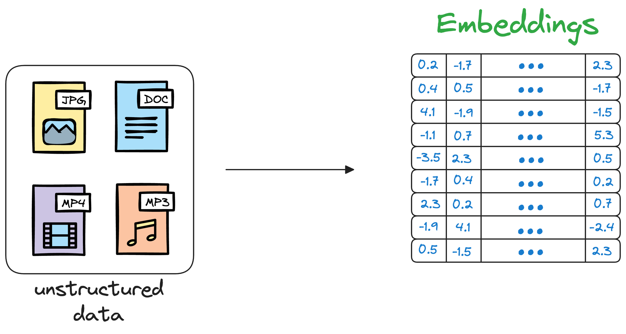
Each data point, whether a word, a document, an image, or any other entity, is transformed into a numerical vector using ML techniques (which we shall see ahead).

This numerical vector is called an embedding, and the model is trained in such a way that these vectors capture the essential features and characteristics of the underlying data.

Considering word embeddings, for instance, we may discover that in the embedding space, the embeddings of fruits are found close to each other, which cities form another cluster, and so on.

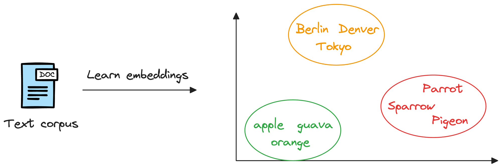
This shows that embeddings can learn the semantic characteristics of entities they represent (provided they are trained appropriately).

Once stored in a vector database, we can retrieve original objects that are similar to the query we wish to run on our unstructured data.

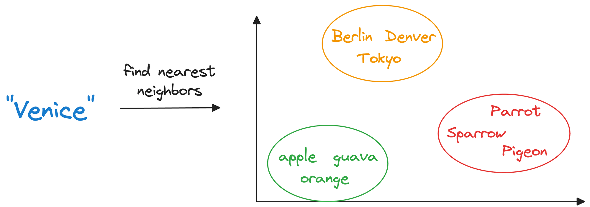
In other words, encoding unstructured data allows us to run many sophisticated operations like similarity search, clustering, and classification over it, which otherwise is difficult with traditional databases.

To exemplify, when an e-commerce website provides recommendations for similar items or searches for a product based on the input query, we’re (in most cases) interacting with vector databases behind the scenes.

Before we get into the technical details, let me give you a couple of intuitive examples to understand vector databases and their immense utility.

Example #1

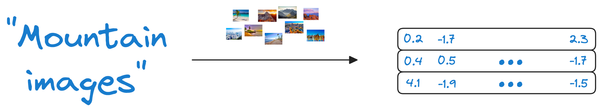
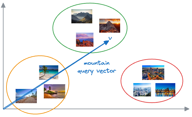
Let's imagine we have a collection of photographs from various vacations we’ve taken over the years. Each photo captures different scenes, such as beaches, mountains, cities, and forests.

Now, we want to organize these photos in a way that makes it easier to find similar ones quickly.

Traditionally, we might organize them by the date they were taken or the location where they were shot.

However, we can take a more sophisticated approach by encoding them as vectors.

More specifically, instead of relying solely on dates or locations, we could represent each photo as a set of numerical vectors that capture the essence of the image.

Let’s say we use an algorithm that converts each photo into a vector based on its color composition, prominent shapes, textures, people, etc.

Each photo is now represented as a point in a multi-dimensional space, where the dimensions correspond to different visual features and elements in the image.

Now, when we want to find similar photos, say, based on our input text query, we encode the text query into a vector and compare it with image vectors.

Photos that match the query are expected to have vectors that are close together in this multi-dimensional space.

Suppose we wish to find images of mountains.

In that case, we can quickly find such photos by querying the vector database for images close to the vector representing the input query.

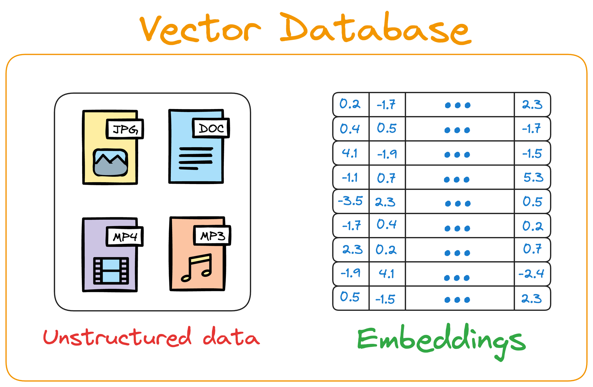
A point to note here is that a vector database is NOT just a database to keep track of embeddings.

Instead, it maintains both the embeddings and the raw data which generated those embeddings.

Why is that necessary, you may wonder?

Considering the above image retrieval task again, if our vector database is only composed of vectors, we would also need a way to reconstruct the image because that is what the end-user needs.

When a user queries for images of mountains, they would receive a list of vectors representing similar images, but without the actual images.

By storing both the embeddings (the vectors representing the images) and the raw image data, the vector database ensures that when a user queries for similar images, it not only returns the closest matching vectors but also provides access to the original images.

Example #2

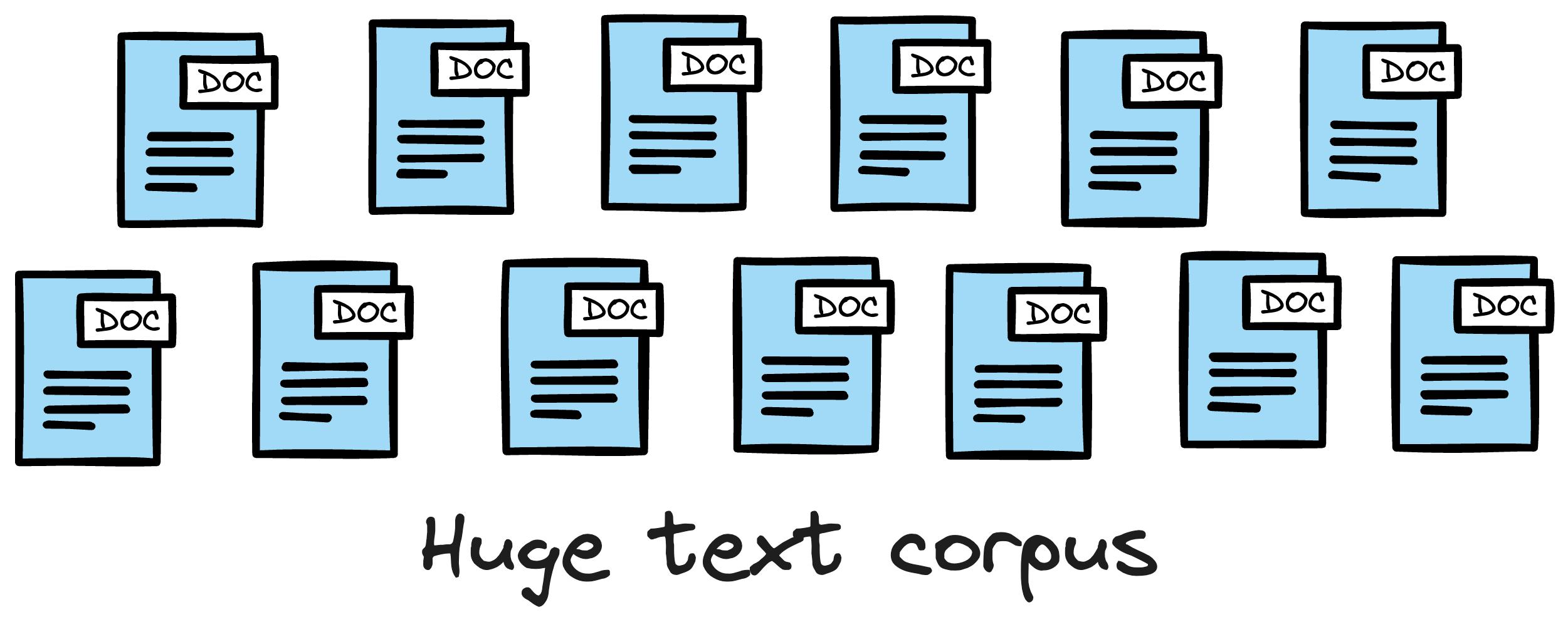
In this example, consider an all-text unstructured data, say thousands of news articles, and we wish to search for an answer from that data.

Traditional search methods rely on exact keyword search, which is entirely a brute-force approach and does not consider the inherent complexity of text data.

In other words, languages are incredibly nuanced, and each language provides various ways to express the same idea or ask the same question.

For instance, a simple inquiry like "What's the weather like today?" can be phrased in numerous ways, such as "How's the weather today?", "Is it sunny outside?", or "What are the current weather conditions?".

This linguistic diversity makes traditional keyword-based search methods inadequate.

As you may have already guessed, representing this data as vectors can be pretty helpful in this situation too.

Instead of relying solely on keywords and following a brute-force search, we can first represent text data in a high-dimensional vector space and store them in a vector database.

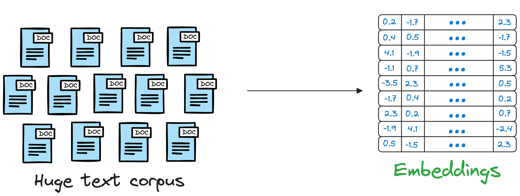
When users pose queries, the vector database can compare the vector representation of the query with that of the text data, even if they don't share the exact same wording.

How to generate embeddings?

At this point, if you are wondering how do we even transform words (strings) into vectors (a list of numbers), let me explain.

We also covered this in a recent newsletter issue here but not in much detail, so let’s discuss those details here.

A Pivotal Moment in NLP Research Which Made Static Embeddings (Almost) Obsolete

Looking back to the pre-Transformer times.

Daily Dose of Data ScienceAvi Chawla

If you already know what embedding models are, feel free to skip this part.

To build models for language-oriented tasks, it is crucial to generate numerical representations (or vectors) for words.

This allows words to be processed and manipulated mathematically and perform various computational operations on words.

The objective of embeddings is to capture semantic and syntactic relationships between words. This helps machines understand and reason about language more effectively.

In the pre-Transformers era, this was primarily done using pre-trained static embeddings.

Essentially, someone would train embeddings on, say, 100k, or 200k common words using deep learning techniques and open-source them.

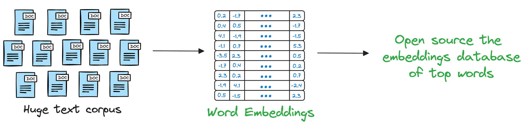
Consequently, other researchers would utilize those embeddings in their projects.

The most popular models at that time (around 2013-2017) were:

• Glove
• Word2Vec
• FastText, etc.

These embeddings genuinely showed some promising results in learning the relationships between words.

For instance, at that time, an experiment showed that the vector operation (King - Man) + Woman returned a vector near the word Queen.

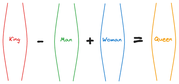
That’s pretty interesting, isn’t it?

In fact, the following relationships were also found to be true:

• Paris - France + Italy ≈ Rome
• Summer - Hot + Cold ≈ Winter
• Actor - Man + Woman ≈ Actress
• and more.

So, while these embeddings captured relative word representations, there was a major limitation.

Consider the following two sentences:

• Convert this data into a table in Excel.
• Put this bottle on the table.

Here, the word “table” conveys two entirely different meanings:

• The first sentence refers to a “data” specific sense of the word “table.”
• The second sentence refers to a “furniture” specific sense of the word “table.”

Yet, static embedding models assigned them the same representation.

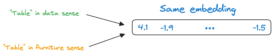
Thus, these embeddings didn’t consider that a word may have different usages in different contexts.

But this was addressed in the Transformer era, which resulted in contextualized embedding models powered by Transformers, such as:

• BERT: A language model trained using two techniques:
  • Masked Language Modeling (MLM): Predict a missing word in the sentence, given the surrounding words.
  • Next Sentence Prediction (NSP).
  • We shall discuss it in a bit more detail shortly.
• DistilBERT: A simple, effective, and lighter version of BERT, which is around 40% smaller:
  • Utilizes a common machine learning strategy called student-teacher theory.
  • Here, the student is the distilled version of BERT, and the teacher is the original BERT model.
  • The student model is supposed to replicate the teacher model’s behavior.
  • If you want to learn how this is implemented practically, we discussed it here:

Model Compression: A Critical Step Towards Efficient Machine Learning

Four critical ways to reduce model footprint and inference time.

Daily Dose of Data ScienceAvi Chawla

• SentenceTransformer: If you read the most recent deep dive on building classification models on ordinal data, we discussed this model there.
  • Essentially, the SentenceTransformer model takes an entire sentence and generates an embedding for that sentence.

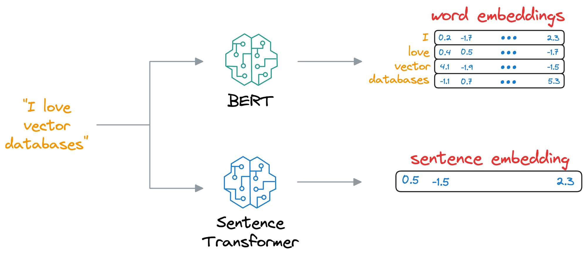
• This differs from the BERT and DistilBERT models, which produce an embedding for all words in the sentence.

There are more models, but we won't go into more detail here, and I hope you get the point.

The idea is that these models are quite capable of generating context-aware representations, thanks to their self-attention mechanism and appropriate training mechanism.

BERT

For instance, if we consider BERT again, we discussed above that it uses the masked language modeling (MLM) technique and next sentence prediction (NSP).

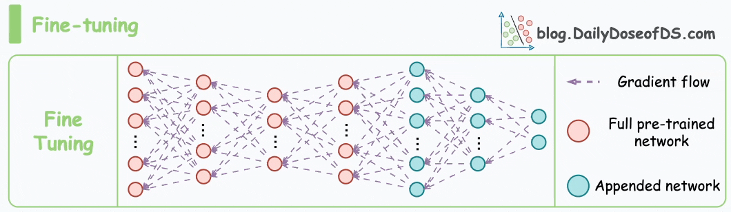
These steps are also called the pre-training step of BERT because they involve training the model on a large corpus of text data before fine-tuning it on specific downstream tasks.

Moving on, let’s see how the pre-training objectives of masked language modeling (MLM) and next sentence prediction (NSP) help BERT generate embeddings.

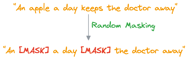
#1) Masked Language Modeling (MLM)

• In MLM, BERT is trained to predict missing words in a sentence. To do this, a certain percentage of words in most (not all) sentences are randomly replaced with a special token, [MASK].

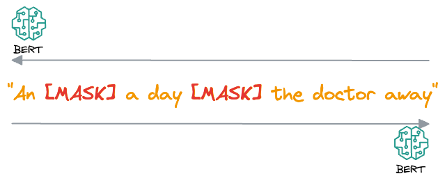
• BERT then processes the masked sentence bidirectionally, meaning it considers both the left and right context of each masked word, that is why the name “Bidirectional Encoder Representation from Transformers (BERT).”

• For each masked word, BERT predicts what the original word is supposed to be from its context. It does this by assigning a probability distribution over the entire vocabulary and selecting the word with the highest probability as the predicted word.

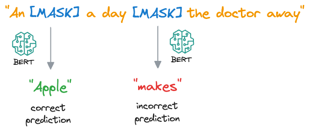
• During training, BERT is optimized to minimize the difference between the predicted words and the actual masked words, using techniques like cross-entropy loss.

#2) Next Sentence Prediction (NSP)

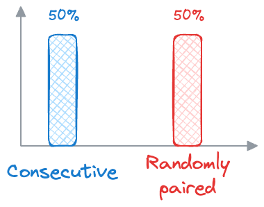
• In NSP, BERT is trained to determine whether two input sentences appear consecutively in a document or whether they are randomly paired sentences from different documents.

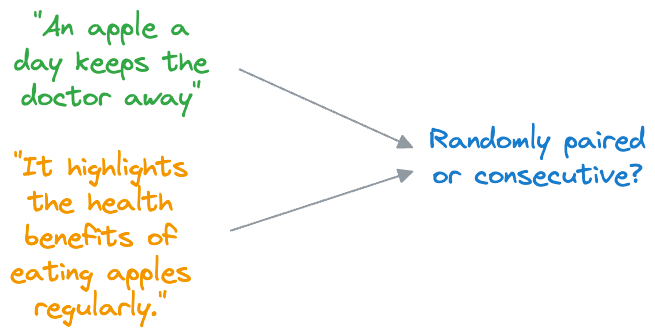
• During training, BERT receives pairs of sentences as input. Half of these pairs are consecutive sentences from the same document (positive examples), and the other half are randomly paired sentences from different documents (negative examples).

• BERT then learns to predict whether the second sentence follows the first sentence in the original document (label 1) or whether it is a randomly paired sentence (label 0).
• Similar to MLM, BERT is optimized to minimize the difference between the predicted labels and the actual labels, using techniques like binary cross-entropy loss.

Now, let's see how these pre-training objectives help BERT generate embeddings:

• MLM: By predicting masked words based on their context, BERT learns to capture the meaning and context of each word in a sentence. The embeddings generated by BERT reflect not just the individual meanings of words but also their relationships with surrounding words in the sentence.
• NSP: By determining whether sentences are consecutive or not, BERT learns to understand the relationship between different sentences in a document. This helps BERT generate embeddings that capture not just the meaning of individual sentences but also the broader context of a document or text passage.

With consistent training, the model learns how different words relate to each other in sentences. It learns which words often come together and how they fit into the overall meaning of a sentence.

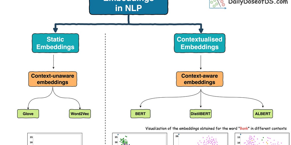
This learning process helps BERT create embeddings for words and sentences, which are contextualized, unlike earlier embeddings like Glove and Word2Vec:

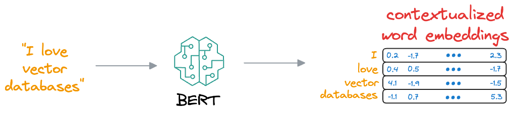
Contextualized means that the embedding model can dynamically generate embeddings for a word based on the context they were used in.

As a result, if a word would appear in a different context, the model would return a different representation.

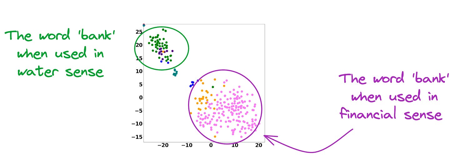
This is precisely depicted in the image below for different uses of the word Bank.

For visualization purposes, the embeddings have been projected into 2d space using t-SNE.

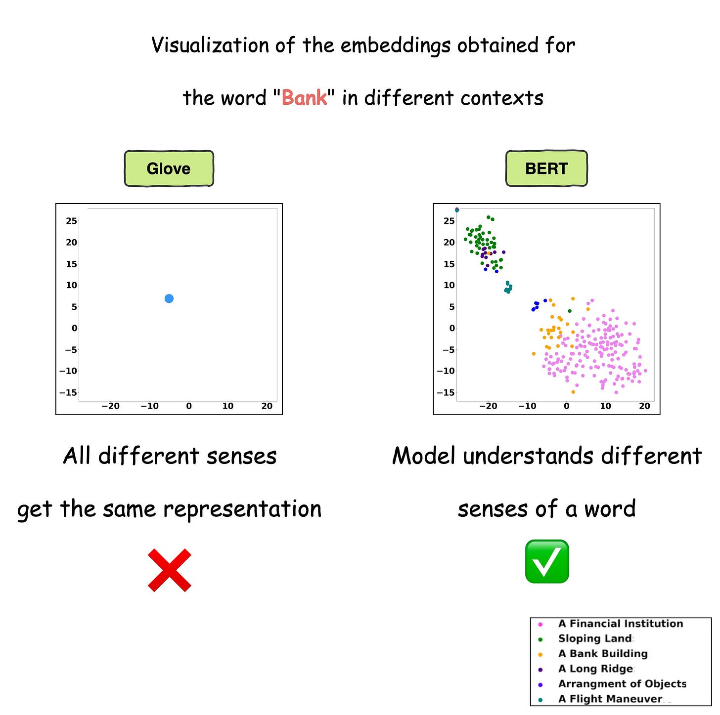
As depicted above, the static embedding models — Glove and Word2Vec produce the same embedding for different usages of a word.

However, contextualized embedding models don’t.

In fact, contextualized embeddings understand the different meanings/senses of the word “Bank”:

• A financial institution
• Sloping land
• A Long Ridge, and more.

As a result, these contextualized embedding models address the major limitations of static embedding models.

The point of the above discussion is that modern embedding models are quite proficient at the encoding task.

As a result, they can easily transform documents, paragraphs, or sentences into a numerical vector that captures its semantic meaning and context.

Querying a vector database

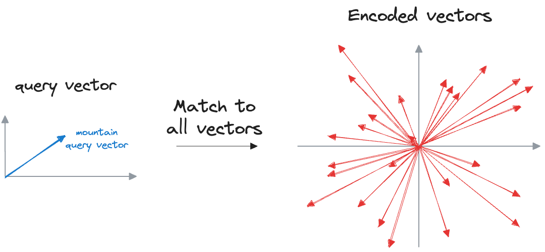
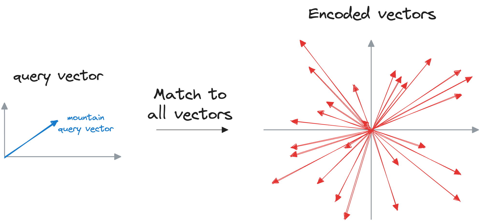
In the last to last sub-section, we provided an input query, which was encoded, and then we searched the vector database for vectors that were similar to the input vector.

In other words, the objective was to return the nearest neighbors as measured by a similarity metric, which could be:

• Euclidean distance (the lower the metric, the more the similarity).
• Manhattan distance (the lower the metric, the more the similarity).
• Cosine similarity (the more the metric, the more the similarity).

The idea resonates with what we do in a typical k-nearest neighbors (kNN) setting.

We can match the query vector across the already encoded vectors and return the model similar ones.

The problem with this approach is that to find, say, only the first nearest neighbor, the input query must be matched across all vectors stored in the vector database.

This is computationally expensive, especially when dealing with large datasets, which may have millions of data points. As the size of the vector database grows, the time required to perform a nearest neighbor search increases proportionally.

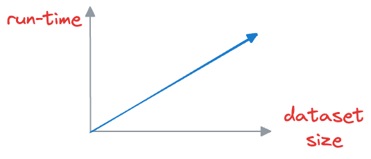
But in scenarios where real-time or near-real-time responses are necessary, this brute-force approach becomes impractical.

In fact, this problem is also observed in typical relational databases. If we were to fetch rows that match a particular criteria, the whole table must be scanned.

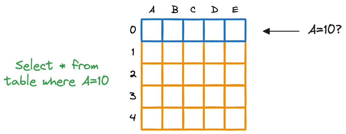
Indexing the database provides a quick lookup mechanism, especially in cases where near real-time latency is paramount.

More specifically, when columns used in WHERE clauses or JOIN conditions are indexed, it can significantly speed up query performance.

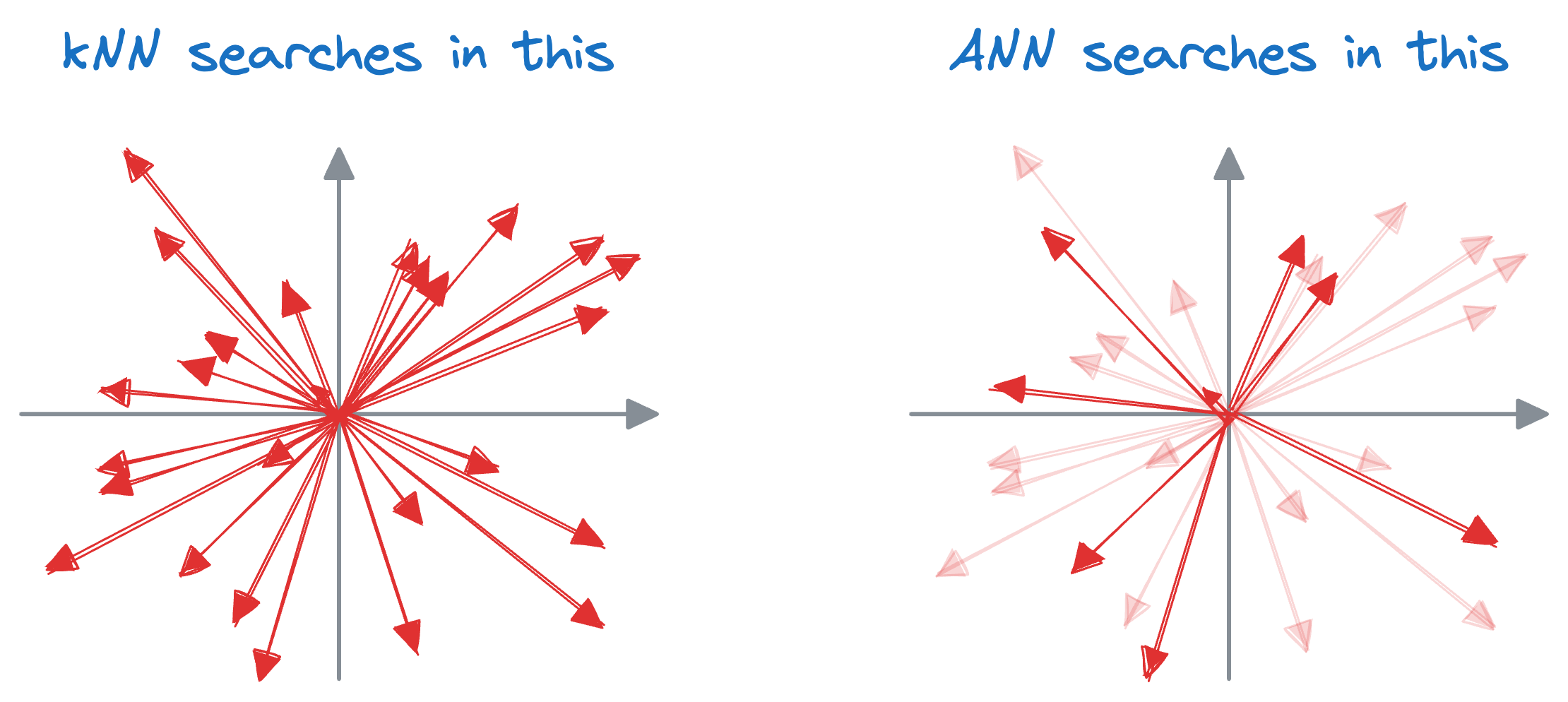
A similar idea of indexing is also utilized in vector databases, which results in something we call an approximate nearest neighbor (ANN), which is quite self-explanatory, isn't it?

Well, the core idea is to have a tradeoff between accuracy and run time. Thus, approximate nearest neighbor algorithms are used to find the closest neighbors to a data point, though these neighbors may not always be the closest neighbors.

That is why they are also called non-exhaustive search algorithms.

The motivation is that when we use vector search, exact matches aren't absolutely necessary in most cases.

Approximate nearest neighbor (ANN) algorithms utilize this observation and compromise a bit of accuracy for run-time efficiency.

Thus, instead of exhaustively searching through all vectors in the database to find the closest matches, ANN algorithms provide fast, sub-linear time complexity solutions that yield approximate nearest neighbors.

Let’s discuss these techniques in the next section!

Approximate nearest neighbors (ANN)

While approximate nearest neighbor algorithms may sacrifice a certain degree of precision compared to exact nearest neighbor methods, they offer significant performance gains, particularly in scenarios where real-time or near-real-time responses are required.

The core idea is to narrow down the search space for the query vector, thereby improving the run-time performance.

The search space is reduced with the help of indexing. There are five popular indexing strategies here.

Let’s go through each of them.

#1) Flat Index

Flat index is another name for the brute-force search we saw earlier, which is also done by KNN. Thus, all vectors are stored in a single index structure without any hierarchical organization.

That is why this indexing technique is called “flat” – it involves no indexing strategy, and stores the data vectors as they are, i.e., in a ‘flat’ data structure.

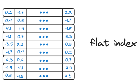
As it searches the entire vector database, it delivers the best accuracy of all indexing methods we shall see ahead. However, this approach is incredibly slow and impractical.

Nonetheless, I wouldn’t recommend adopting any other sophisticated approach over a flat index when the data conditions are favorable, such as having only a few data points to search over and a low-dimensional dataset.

But, of course, not all datasets are small, and using a flat index is impractical in most real-life situations.

Thus, we need more sophisticated approaches to index our vectors in the vector database.

#2) Inverted File Index

IVF is probably one of the most simple and intuitive indexing techniques. While it is commonly used in text retrieval systems, it can be adapted to vector databases for approximate nearest neighbor searches.

Here’s how!

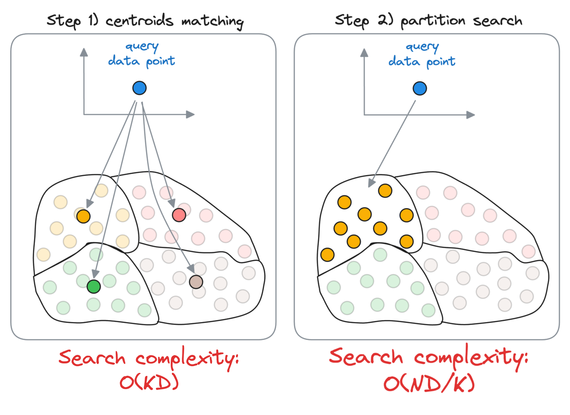
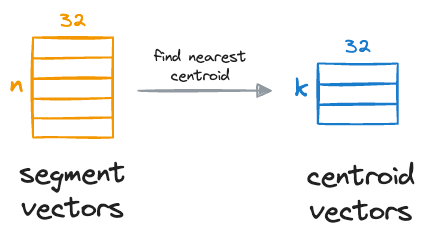
Given a set of vectors in a high-dimensional space, the idea is to organize them into different partitions, typically using clustering algorithms like k-means.

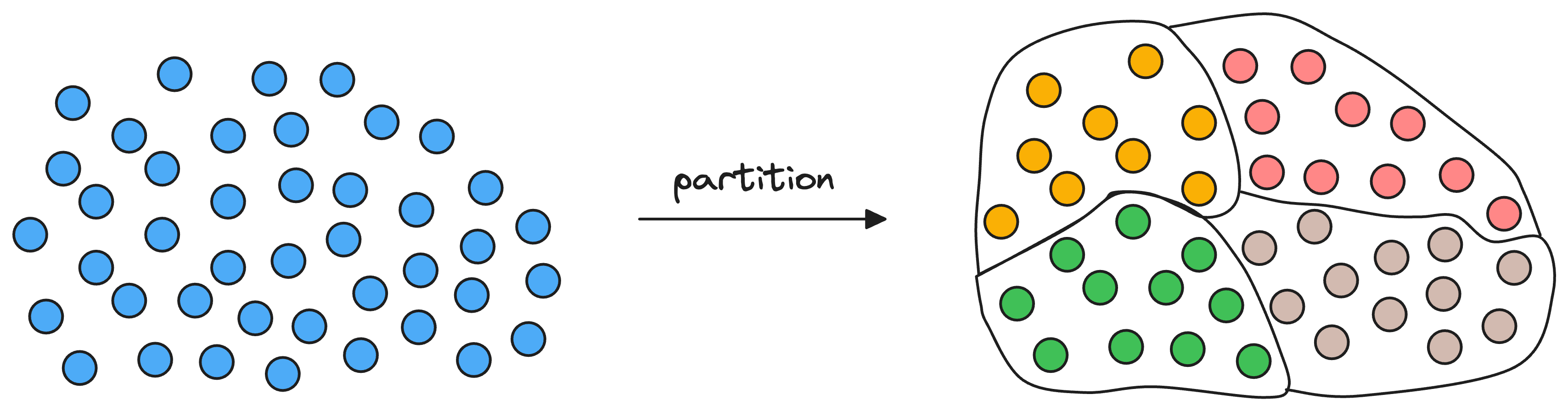
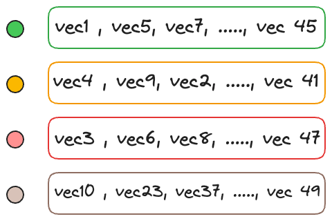
As a result, each partition has a corresponding centroid, and every vector gets associated with only one partition corresponding to its nearest centroid.

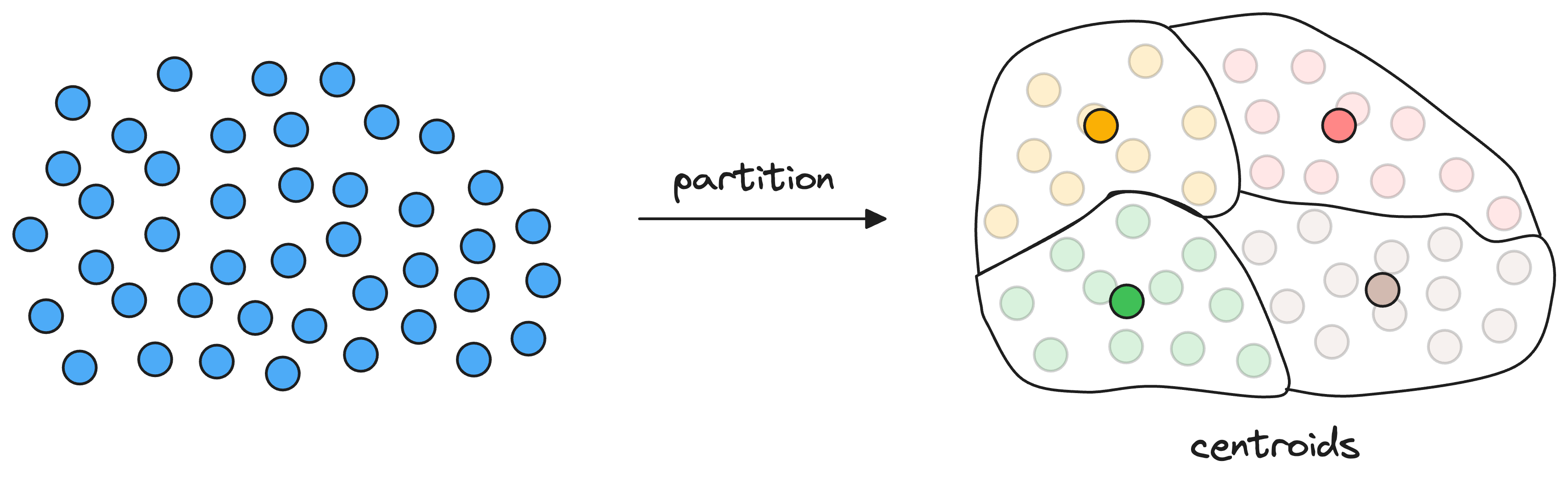
Thus, every centroid maintains information about all the vectors that belong to its partition.

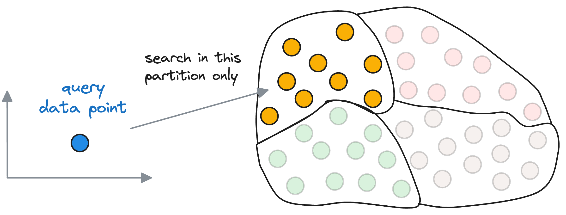
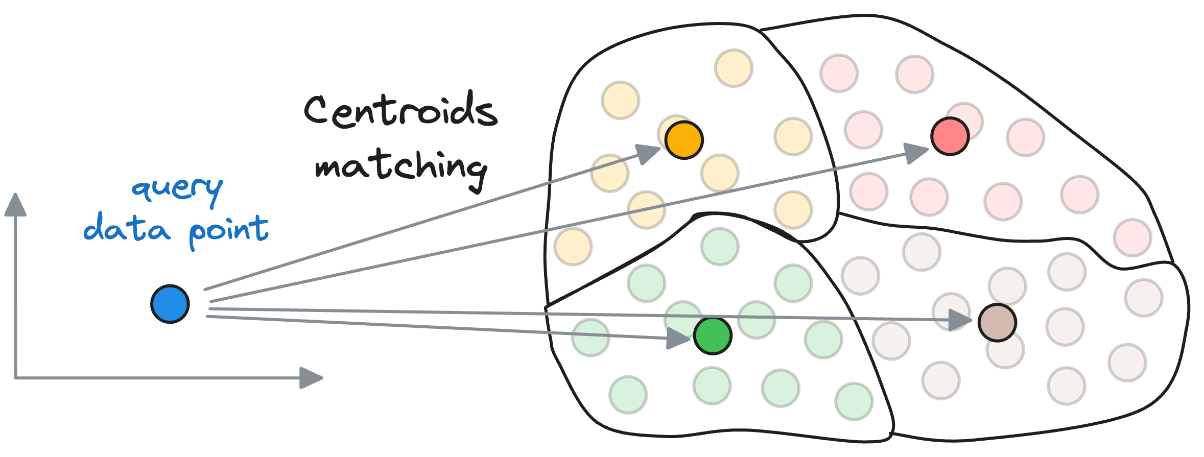
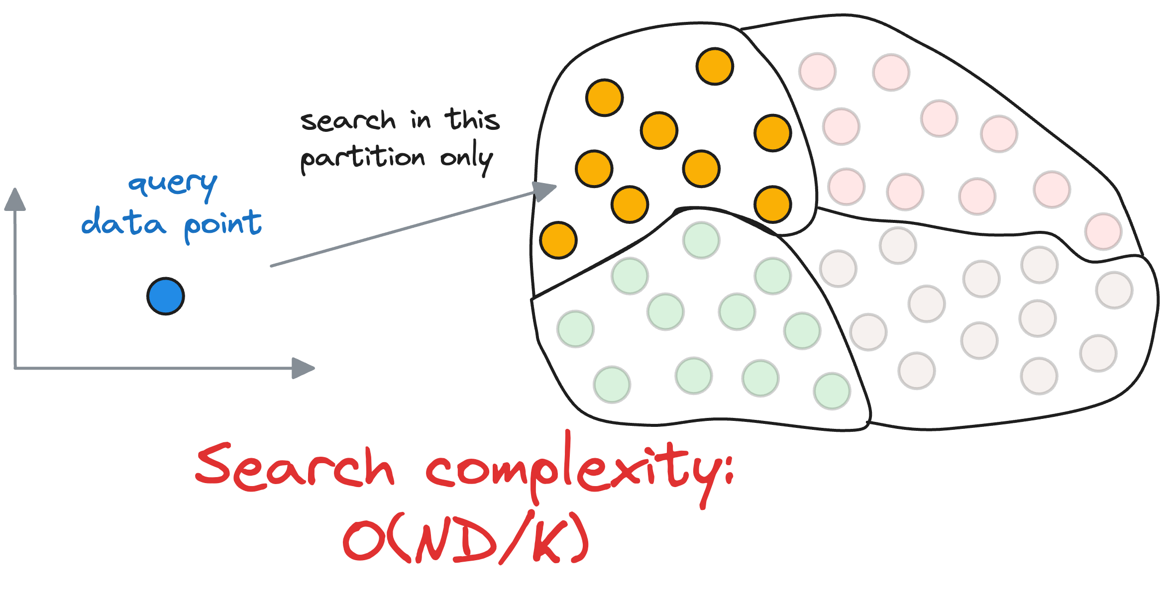
When searching for the nearest vector to the query vector, instead of searching across all vectors, we first find the closest centroid to the query vector.

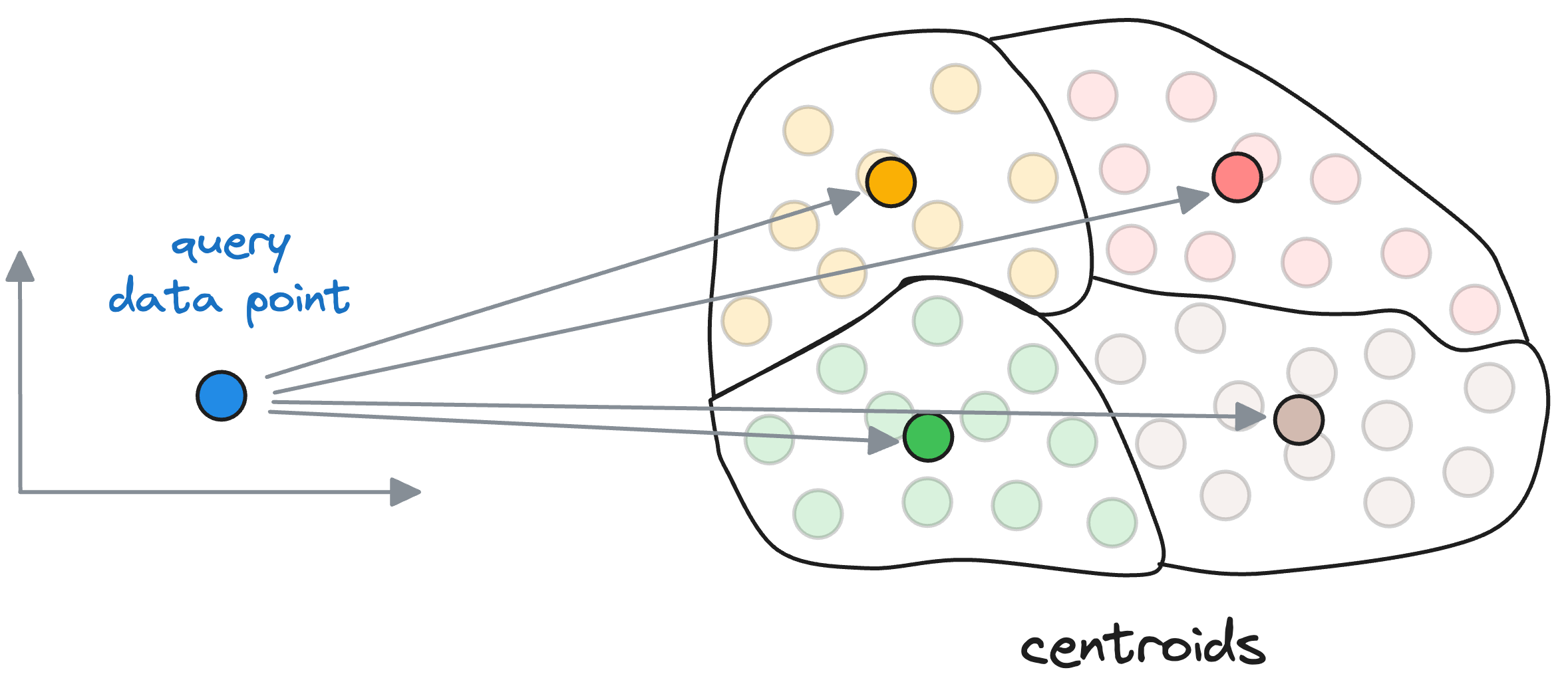
The nearest neighbor is then searched in only those vectors that belong to the partition of the closest centroid found above.

Let’s estimate the search run-time difference it provides over using a flat index.

To reiterate, in flat-index, we compute the similarity of the query vector with all the vectors in the vector database.

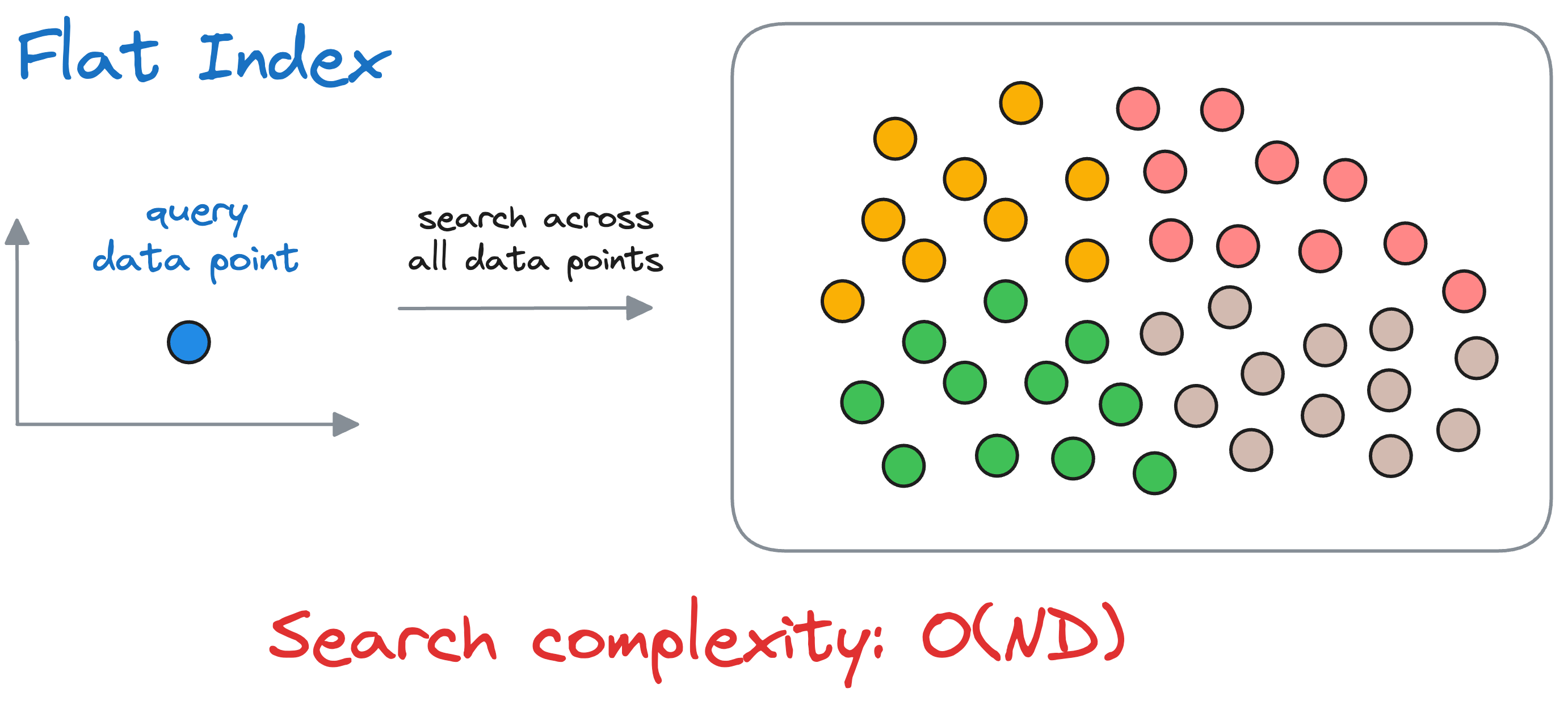
If we have $N$ vectors and each vector is $D$ dimensional, the run-time complexity is $O(ND)$ to find the nearest vector.

Compare it to the Inverted File Index, wherein, we first compute the similarity of the query vector with all the centroids obtained using the clustering algorithm.

Let’s say there are $k$ centroids, a total of $N$ vectors, and each vector is $D$ dimensional.

Also, for simplicity, let’s say that the vectors are equally distributed across all partitions. Thus, each partition will have $\frac{N}{k}$ data points.

First, we compute the similarity of the query vector with all the centroids, whose run-time complexity is $O(kD)$.

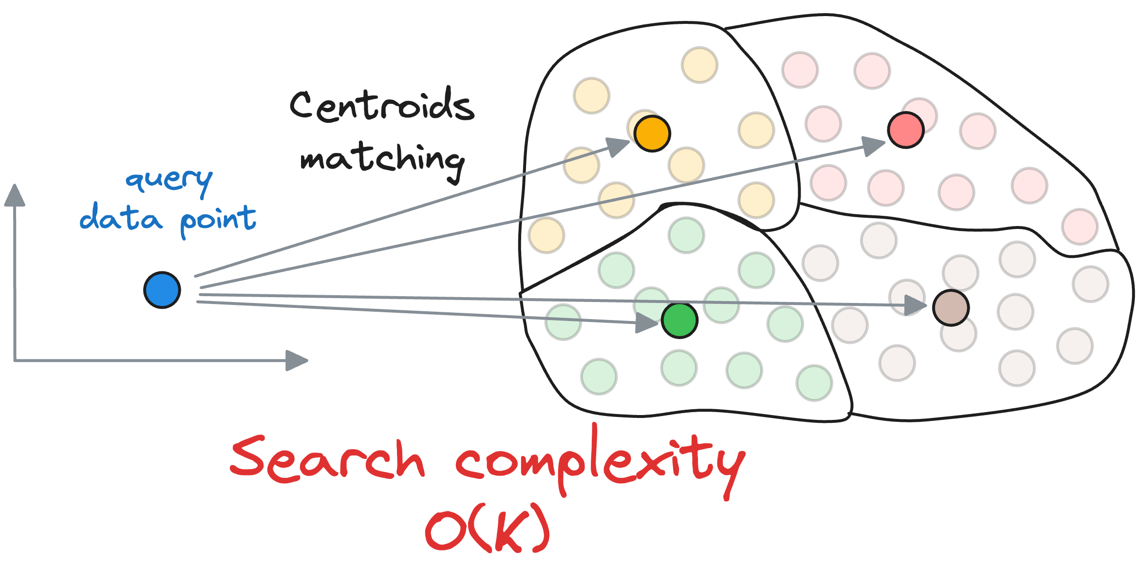
Next, we compute the similarity of the query vector to the data points that belong to the centroid’s partition, with a run-time complexity of $O(\frac{ND}{k})$.

Thus, the overall run-time complexity comes out to be $O(kD+\frac{ND}{k})$.

To get some perspective, let’s assume we have 10M vectors in the vector databases and divide that into $k=100$ centroids. Thus, each partition is expected to have roughly 1 lakh data points.

In the flat index, we shall compare the input query across all data points – 10M.

In IVF, first, we shall compare the input query across all centroids (100), and then compare it to the vectors in the obtained partition (100k). Thus, the total comparisons, in this case, will be 100,050, nearly 100 times faster.

Of course, it is essential to note that if some vectors are actually close to the input vector but still happen to be in the neighboring partition, we will miss them.

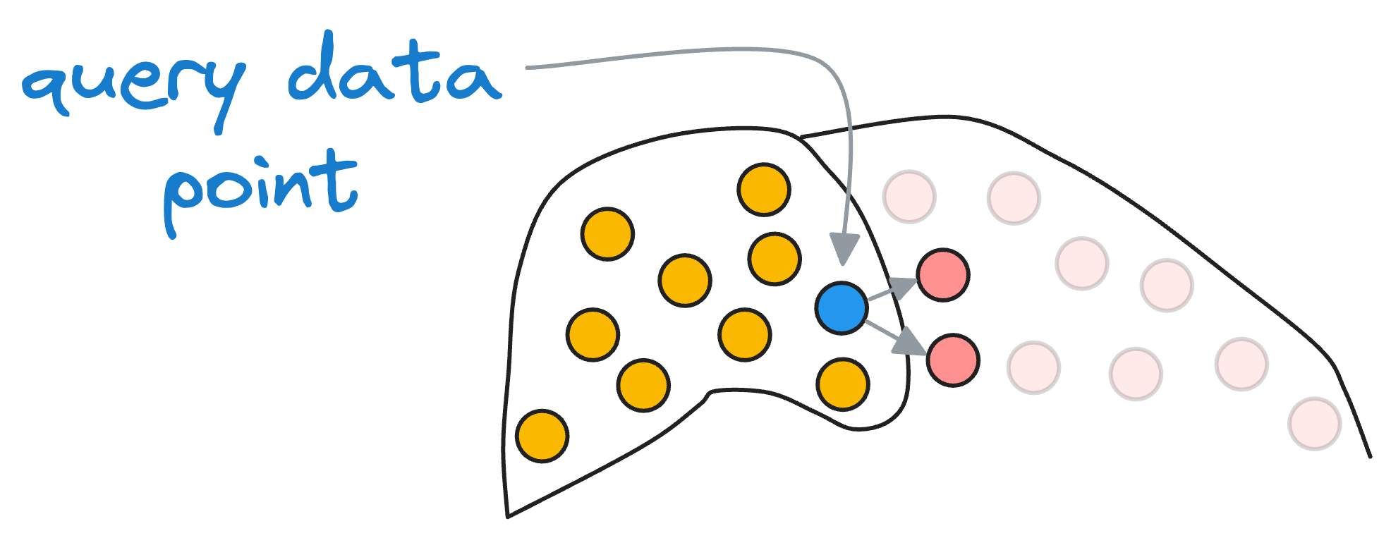
But recalling our objective, we were never aiming for the best solution but an approximate best (that's why we call it “approximate nearest neighbors”), so this accuracy tradeoff is something we willingly accept for better run-time performance.

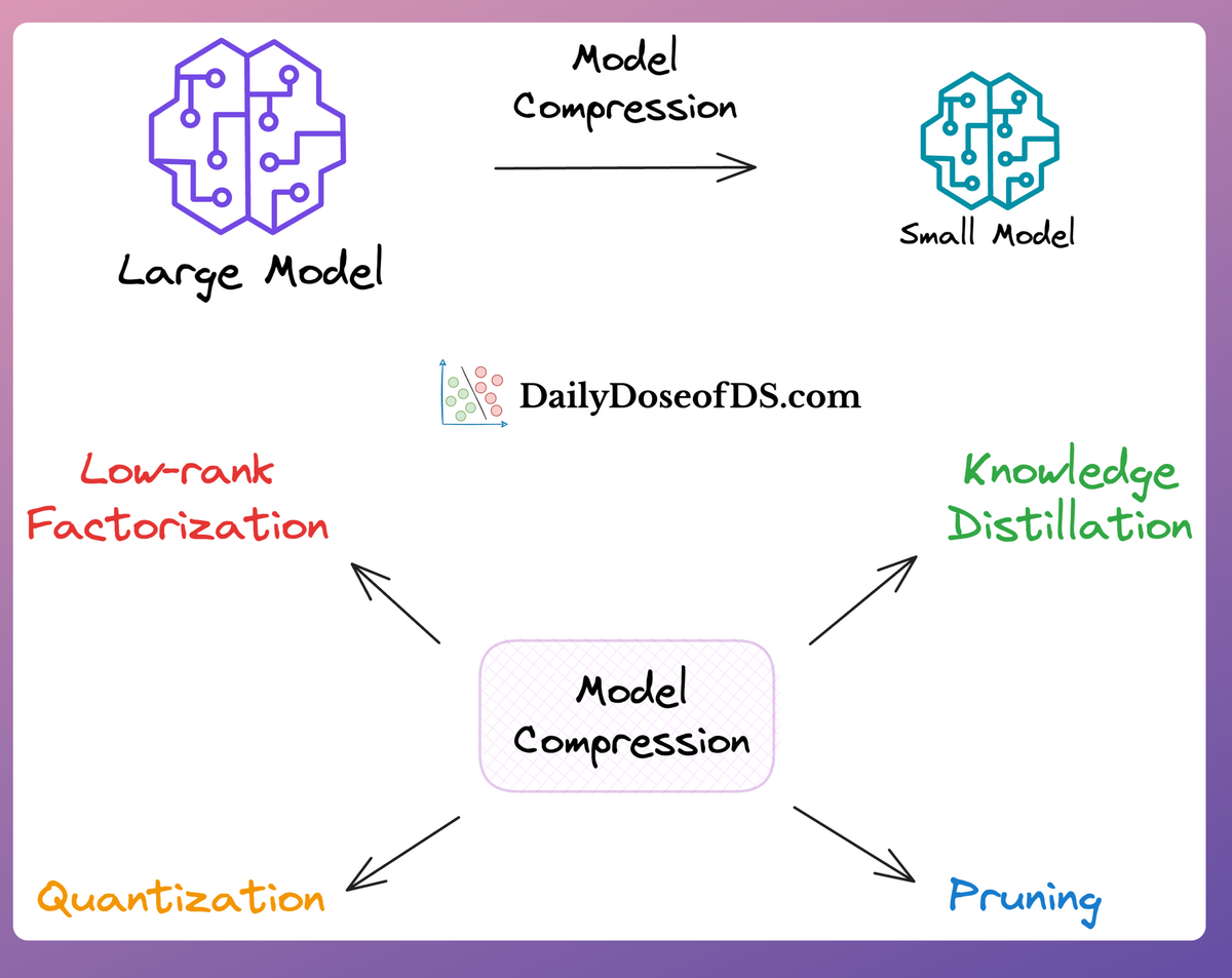
In fact, if you remember the model compression deep dive, we followed the same idea there as well:

Model Compression: A Critical Step Towards Efficient Machine Learning

Four critical ways to reduce model footprint and inference time.

Daily Dose of Data ScienceAvi Chawla

#3) Product Quantization

The idea of quantization in general refers to compressing the data while preserving the original information.

Thus, Product Quantization (PQ) is a technique used for vector compression for memory-efficient nearest neighbor search.

Let’s understand how it works in detail.

Step 1) Create data segments

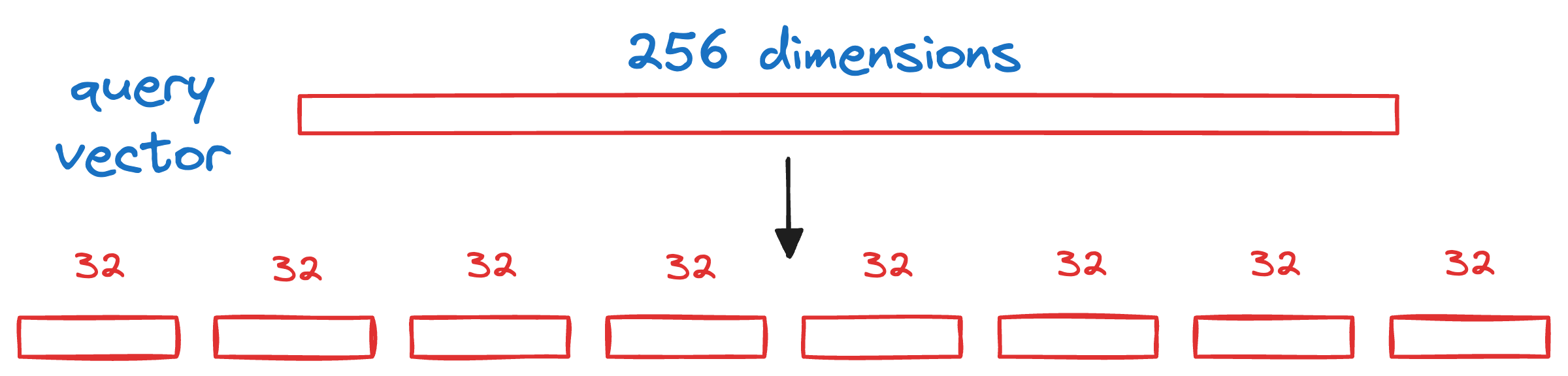
Say we have some vectors, and each vector is 256-dimensional. Assuming each dimension is represented by a number that takes 32 bits, the memory consumed by each vector would be 256 x 32 bits = 8192 bits.

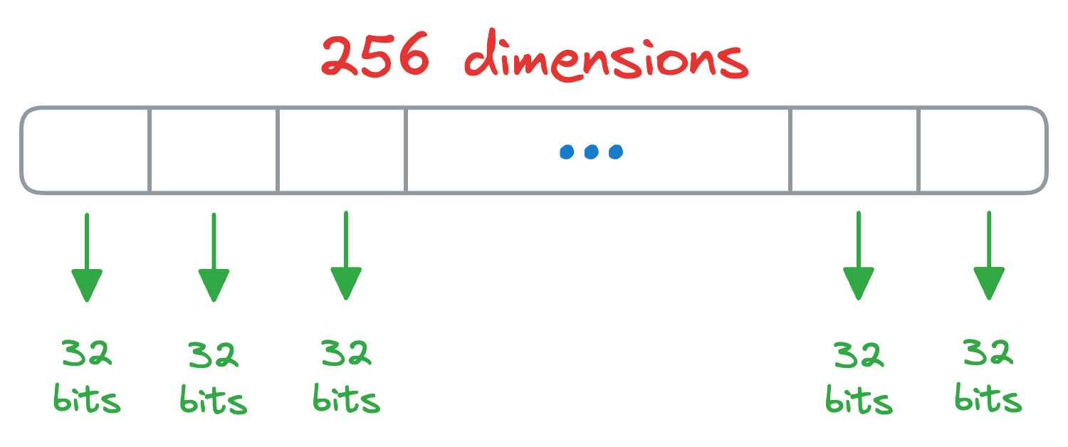
In Product Quantization (PQ), we first split all vectors into sub-vectors. A demonstration is shown below, where we split the vector into M (a parameter) segments, say 8:

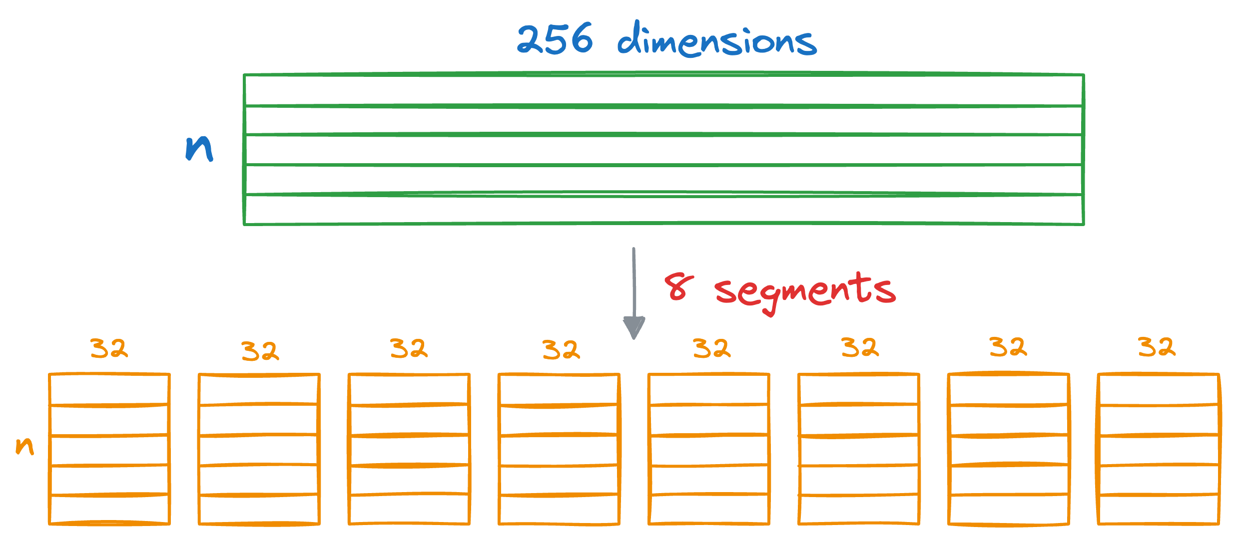
As a result, each segment will be 32-dimensional.

Step 2) Run KMeans

Next, we run KMeans on each segment separately, which will generate k centroids for each segment.

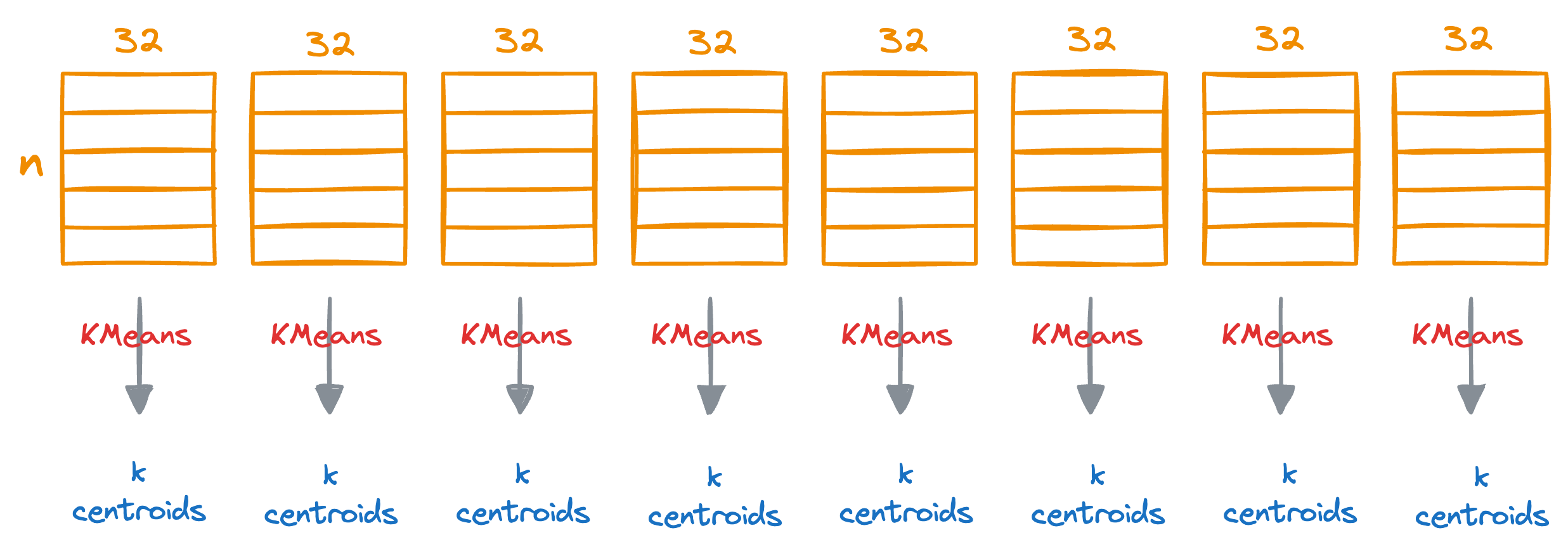
Do note that each centroid will represent the centroid for the subspace (32 dimensions) but not the entire vector space (256 dimensions in this demo).

For instance, if k=100, this will generate 100*8 centroids in total.

Training complete.

Step 3) Encode vectors

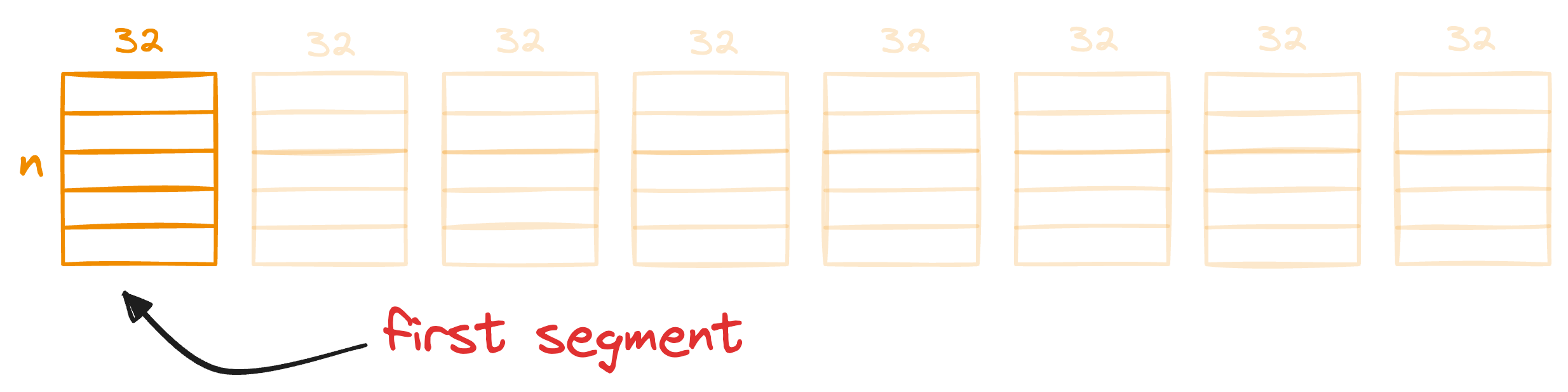
Next, we move to the encoding step.

The idea is that for each segment of a vector in the entire database, we find the nearest centroid from the respective segment, which has k centroids that were obtained in the training step above.

For instance, consider the first segment of the 256-dimensional data we started with:

We compare these segment vectors to the corresponding k centroids and find the nearest centroid for all segment vectors:

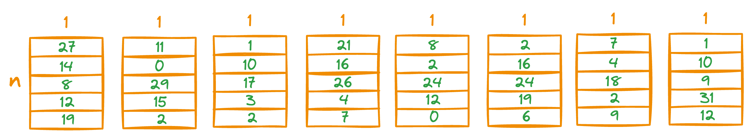
After obtaining the nearest centroid for each vector segment, we replace the entire segment with a unique centroid ID, which can be thought of as indices (a number from 0 to k-1) of the centroids in that sub-space.

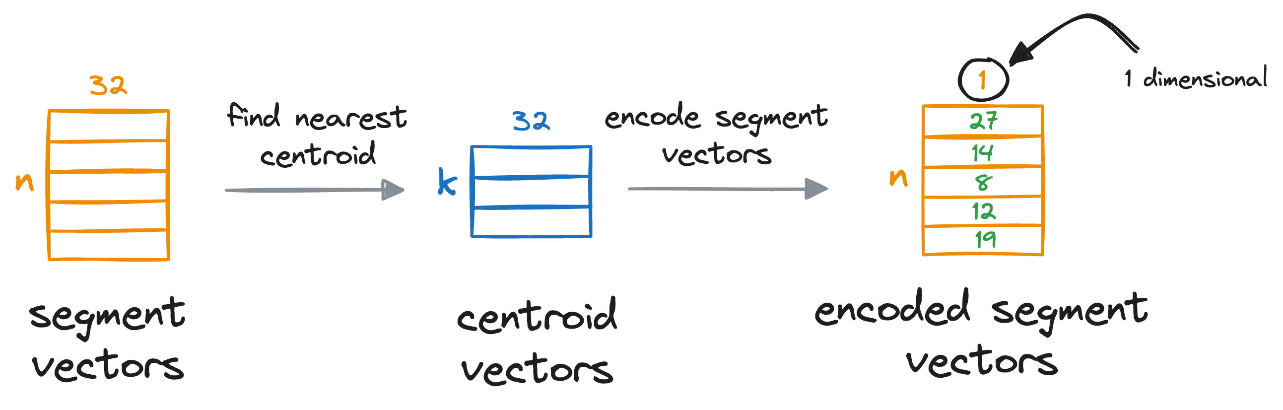
We do see for all individual segments of the vectors:

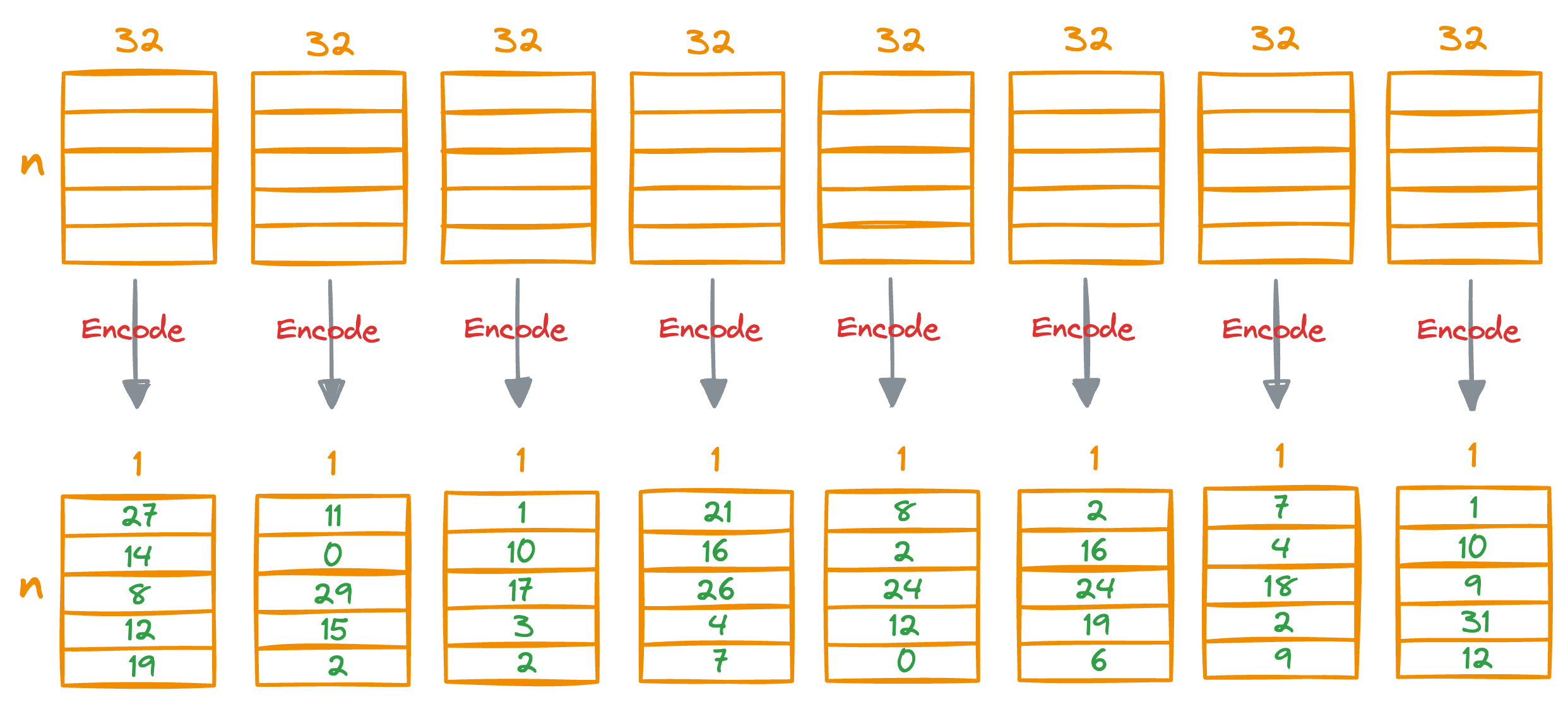
This provides us with a quantized (or compressed) representation of all vectors in the vector database, which is composed of centroid IDs, and they are also known as PQ codes.

To recall, what we did here is that we’ve encoded all the vectors in the vector database with a vector of centroid IDs, which is a number from 0 to k-1, and every dimension now only consumes 8 bits of memory.

As there are 8 segments, total memory consumed is 8*8=64 bits, which is 128 times lower memory usage than what we had earlier – 8192 bits.

The memory saving scales immensely well when we are dealing with millions of vectors.

Of course, the encoded representation isn’t entirely accurate, but don’t worry about that as it is not that important for us to be perfectly precise on all fronts.

Step 4) Find an approximate nearest neighbor

Now, you might be wondering, how exactly do we search for the nearest neighbor based on the encoded representations?

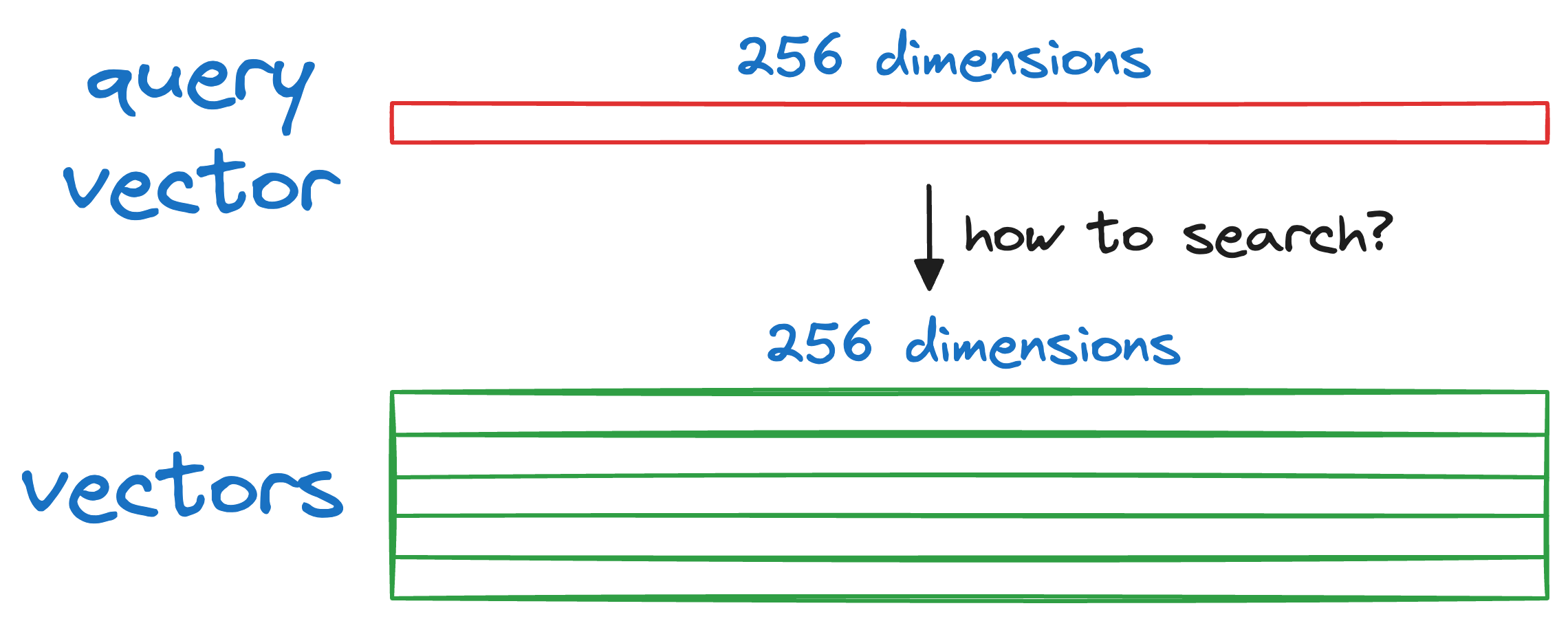
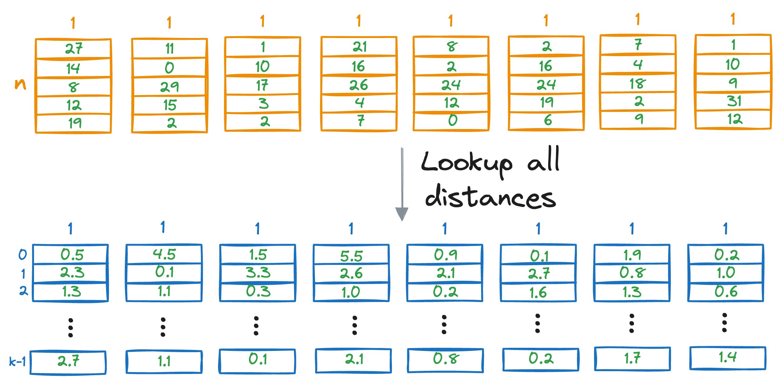
More specifically, given a new query vector Q, we have to find a vector that is most similar (or closest) to Q in our database.

We begin by splitting the query vector Q into M segments, as we did earlier.

Next, we calculate the distance between all segments of the vector Q to all the respective centroids of that segment obtained from the KMeans step above.

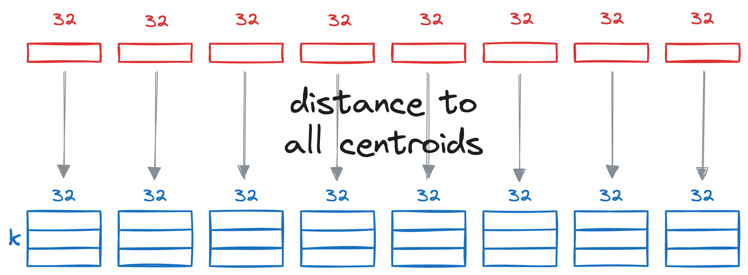
This gives us a distance matrix:

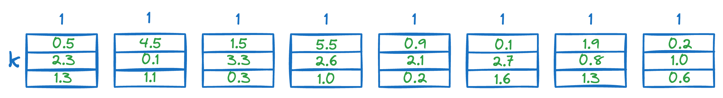
The final step is to estimate the distance of the query vector Q from the vectors in the vector database.

To do this, we go back to the PQ matrix we generated earlier:

Next, we look up the corresponding entries in the distance matrix generated above.

For instance, the first vector in the above PQ matrix is this:

To get the distance of our query vector to this vector, we check the corresponding entries in the distance entries.

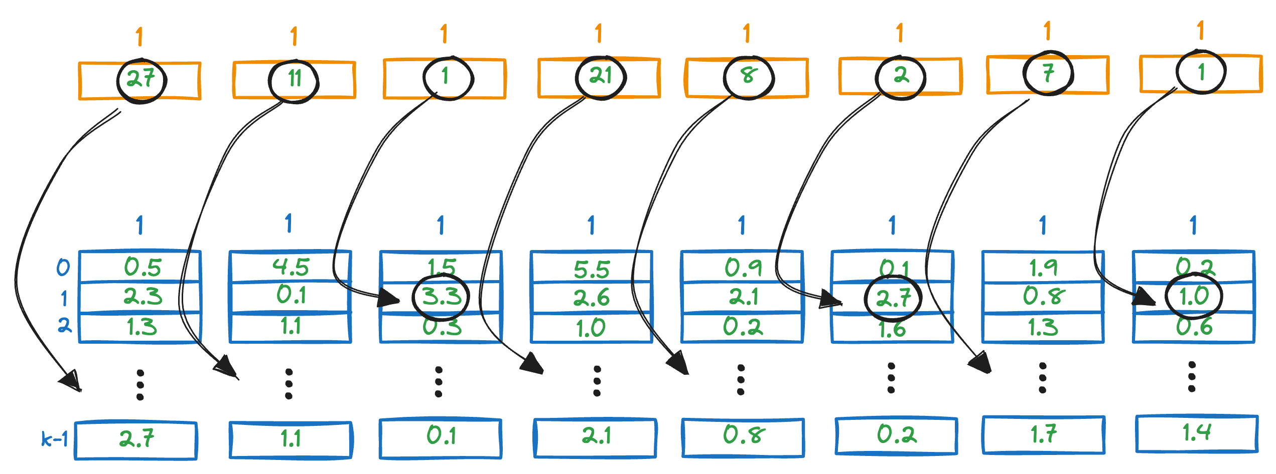
We sum all the segment-wise distances to get a rough estimate of the distance of the query vector Q from all the vectors in the vector database.

We repeat this for all vectors in the database, find the lowest distance, and return the corresponding vectors from the database.

Of course, it is important to note that the above PQ matrix lookup is still a brute-force search. This is because we look up all the distances in the distance matrix for all entries of the PQ matrix.

Moreover, since we are not estimating the vector-to-vector distances but rather vector-to-centroid distances, the obtained values are just approximated distances but not true distances.

Increasing the number of centroids and segments will increase the precision of the approximate nearest neighbor search, but it will also increase the run-time of the search algorithm.

Here’s a summary of the product quantization approach:

• Divide the vectors in the vector database into $M$ segments.
• Run KMeans on each segment. This will give k centroids per segment.
• Encode the vectors in the vector database by replacing each segment of the vector with the centroid ID of the cluster it belongs to. This generates a PQ matrix, which is immensely memory-efficient.
• Next, to determine the approximate nearest neighbor for a query vector Q, generate a distance matrix, whose each entry denotes the distance of a segment of the vector Q to all the centroids.
• Go back to the PQ codes now, and look up the distances in the distance matrix above to get an estimate of the distance between all vectors in the database and the query vector Q. Select the vector with the minimum distance to get the approximate nearest neighbor.

Done!

Approximate nearest neighbor search with product quantization is suitable for medium-sized systems, and it’s pretty clear that there is a tradeoff between precision and memory utilization.

Let’s understand some more effective ways to search for the nearest neighbor.

#4-5) Hierarchical Navigable Small World (HNSW)

HNSW is possibly one of the most effective and efficient indexing methods designed specifically for nearest neighbor searches in high-dimensional spaces.

The core idea is to construct a graph structure, where each node represents a data vector, and edges connect nodes based on their similarity.

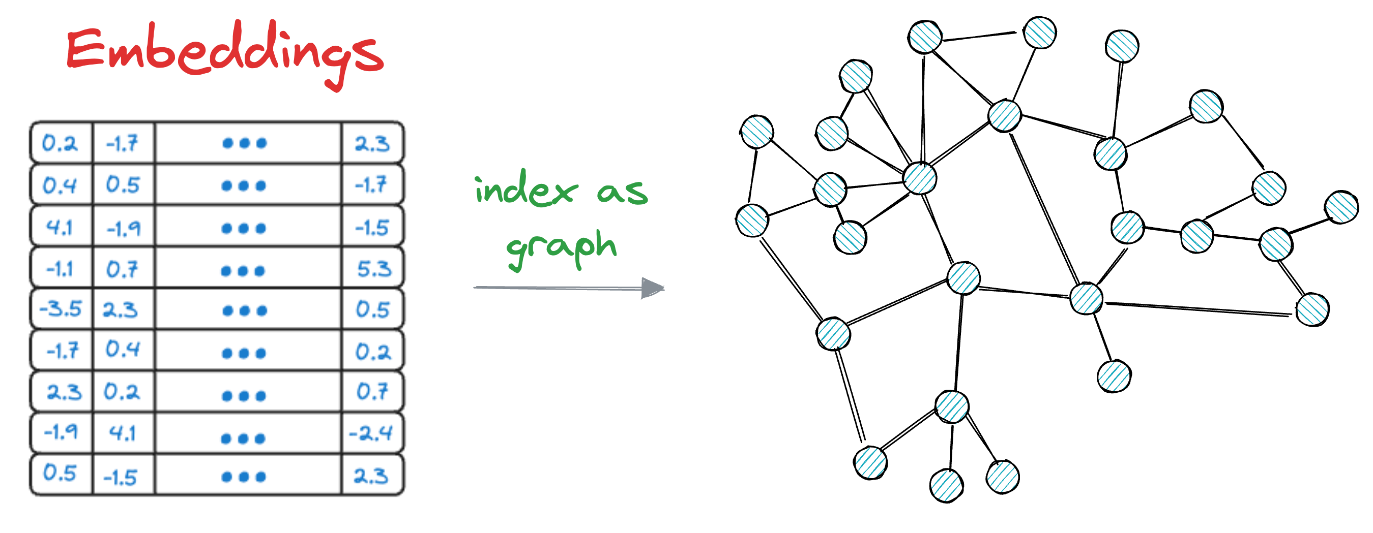
HNSW organizes the graph in such a way that facilitates fast search operations by efficiently navigating through the graph to find approximate nearest neighbors.

But before we understand HNSW, it is crucial to understand NSW (Navigable Small World), which is foundational to the HNSW algorithm.

The upcoming discussion is based on the assumption that you have some idea about graphs.

While we cannot cover them in whole detail, here are some details that will be suffice to understand the upcoming concepts.

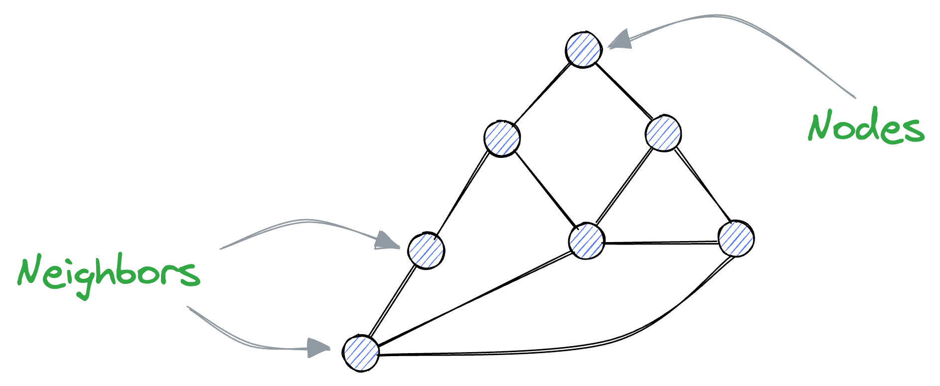
A graph is composed of vertices and edges, where edges connect vertices together. In this context, connected vertices are often referred to as neighbors.

Recalling what we discussed earlier about vectors, we know that similar vectors are usually located close to each other in the vector space.

Thus, if we represent these vectors as vertices of a graph, vertices that are close together (i.e., vectors with high similarity) should be connected as neighbors.

That said, even if two nodes are not directly connected, they should be reachable by traversing other vertices.

This means that we must create a navigable graph.

More formally, for a graph to be navigable, every vertex must have neighbors; otherwise, there will be no way to reach some vertices.

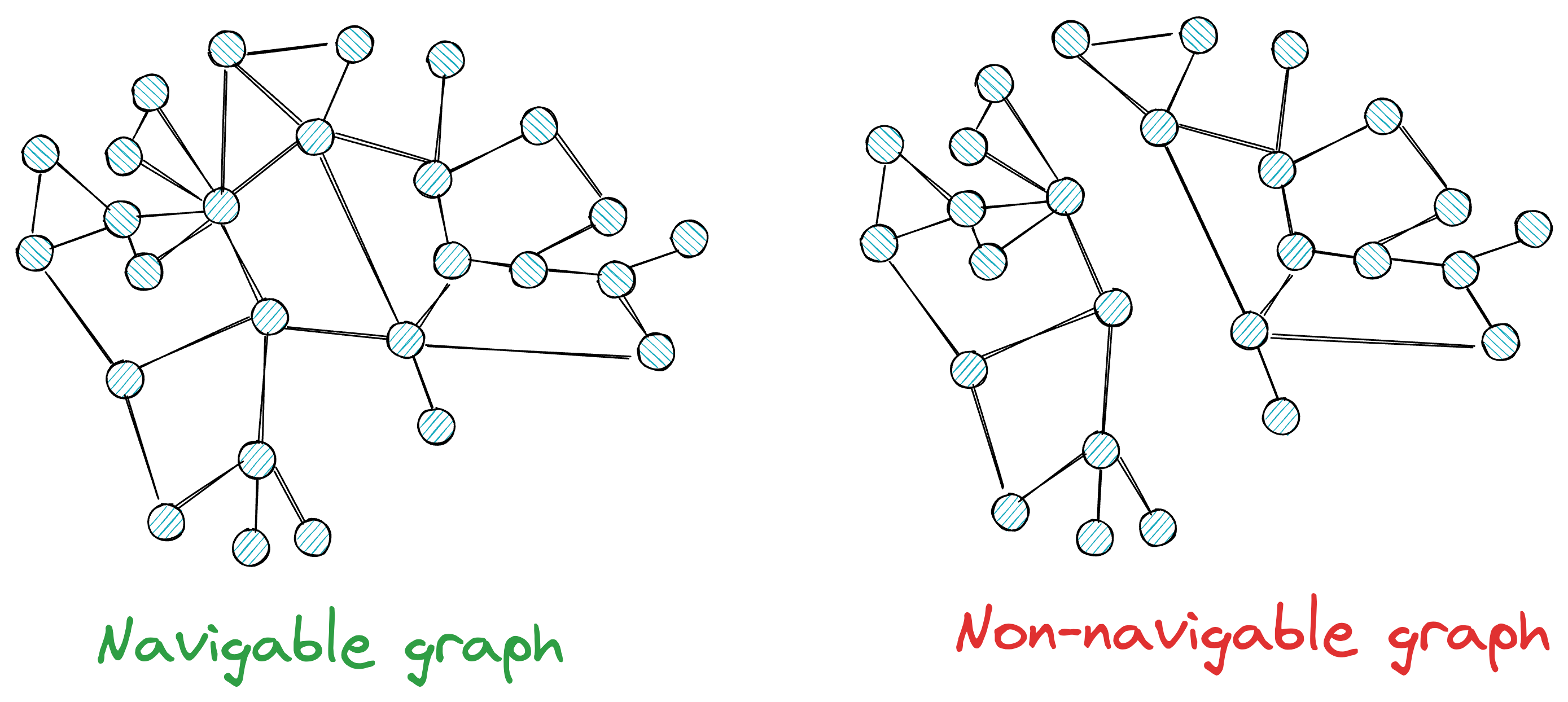
Also, while having neighbors is beneficial for traversal, at the same time, we want to avoid such situations where every node has too many neighbors.

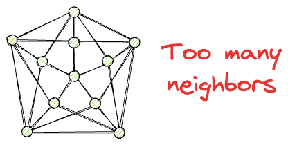
This can be costly in terms of memory, storage, and computational complexity during search time.

Ideally, we want a navigable graph that resembles a small-world network, where each vertex has only a limited number of connections, and the average number of edge traversals between two randomly chosen vertices is low.

This type of graph is efficient for similarity search in large datasets.

If this is clear, we can understand how the Navigable Small World (NSW) algorithm works.

→ Graph construction in NSW

The first step in NSW is graph construction, which we call G.

This is done by shuffling the vectors randomly and constructing the graph by sequentially inserting vertices in a random order.

When adding a new vertex (V) to the graph (G), it shares an edge with K existing vertices in the graph that are closest to it.

This demo will make it more clear.

Say we set K=3.

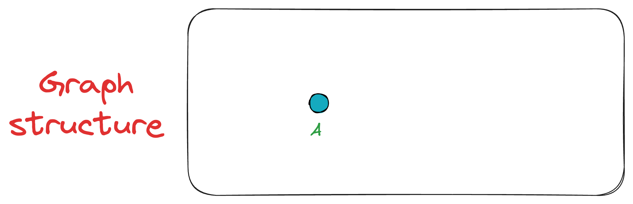
Initially, we insert the first vertex A. As there are no other vertices in the graph at this point, A remains unconnected.

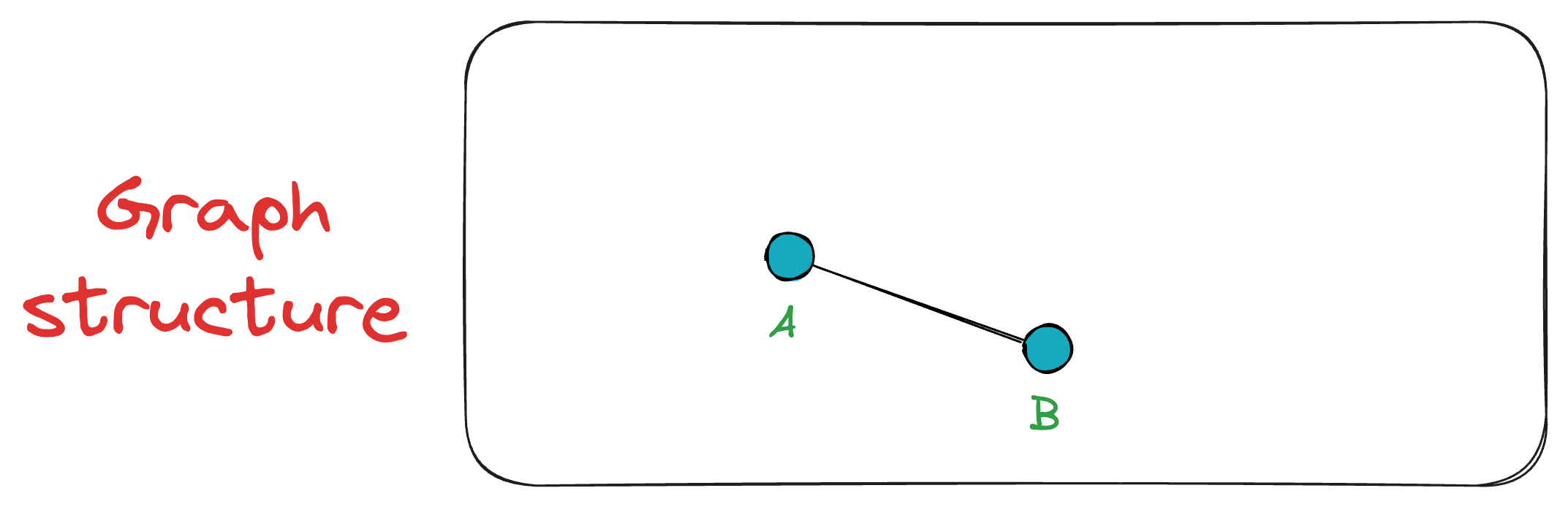
Next, we add vertex B, connecting it to A since A is the only existing vertex, and it will anyway be among the top K closest vertices. Now the graph has two vertices {A, B}.

Next, when vertex C is inserted, it is connected to both A and B. The exact process takes place for the vertex D as well.

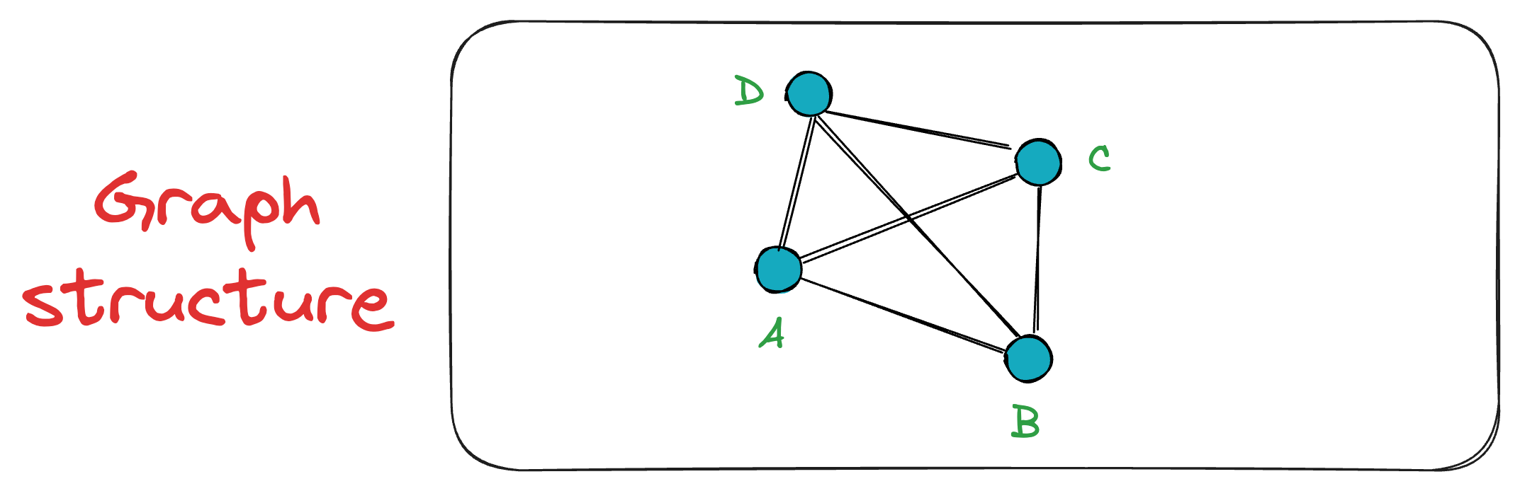
Now, when vertex E is inserted into the graph, it connects only to the K=3 closest vertices, which, in this case, are A, B, and D.

This sequential insertion process continues, gradually building the NSW graph.

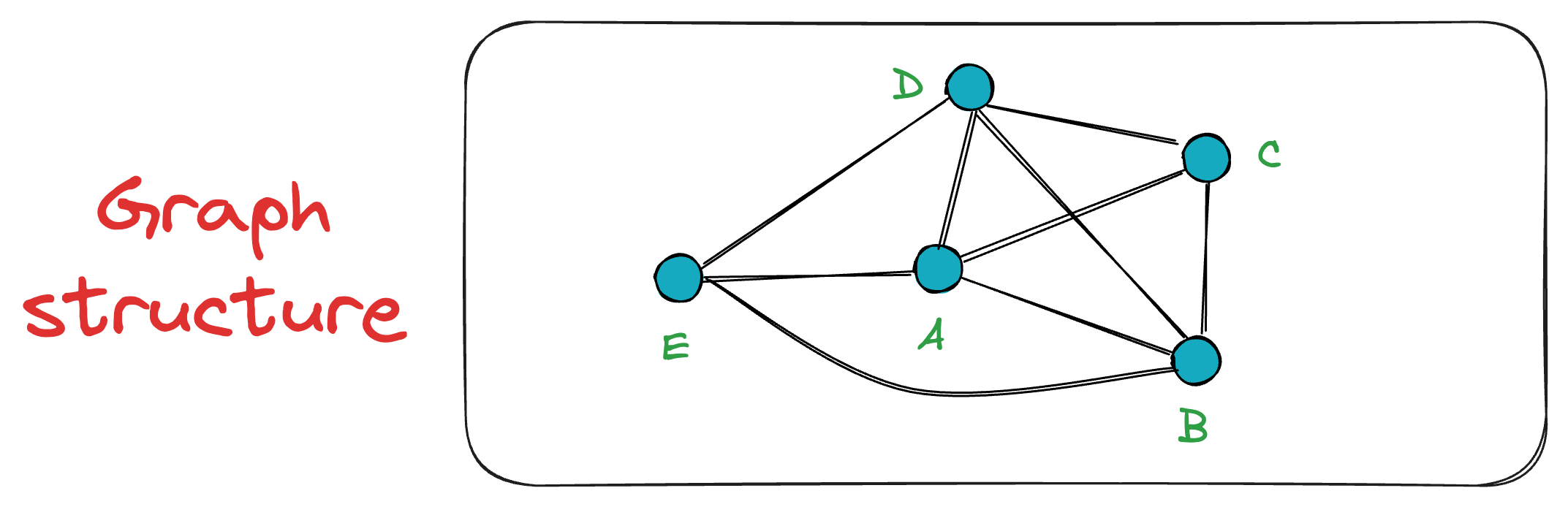
The good thing is that as more and more vertices are added, connections formed in the early stages of the graph constructions may become longer-range links, which makes it easier to navigate long distances in small hops.

This is evident from the following graph, where the connections A — C and B — D span greater distances.

By constructing the graph in this manner, we get an NSW graph, which, most importantly, is navigable.

In other words, any node can be reached from any other node in the graph in some hops.

→ Search in NSW

In the NSW graph (G) constructed above, the search process is conducted using a simple greedy search method that relies on local information at each step.

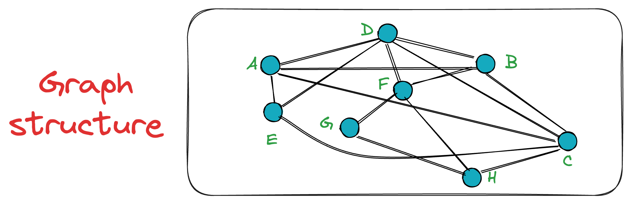
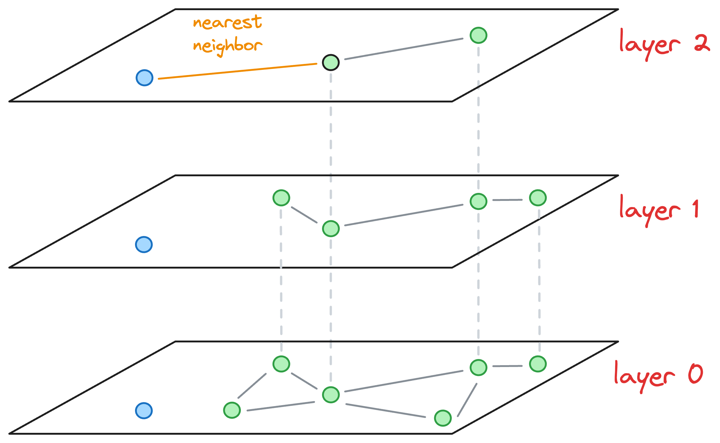
Say we want to find the nearest neighbor to the yellow node in the graph below:

To start the search, an entry point is randomly selected, which is also the beauty of this algorithm. In other words, a key advantage of NSW is that a search can be initiated from any vertex in the graph G.

Let’s choose the node A as the entry point:

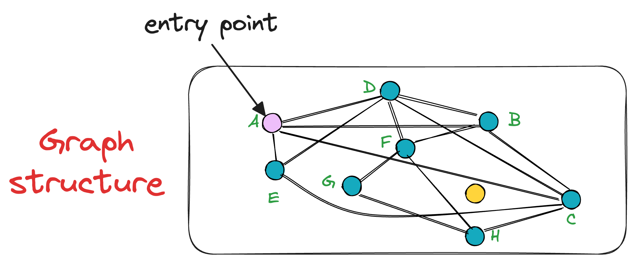
After selecting the initial point, the algorithm iteratively finds a neighbor (i.e., a connected vertex) that is nearest to the query vector Q.

For instance, in this case, the vertex A has neighbors (D, B, C, and E). Thus, we shall compute the distance (or similarity, whatever you chose as a metric) of these 4 neighbors to the query vector Q.

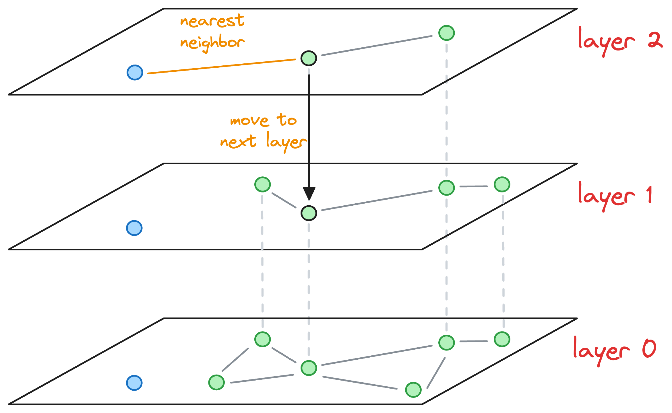
In this case, node C is the closest, so we move to that node C from node A.

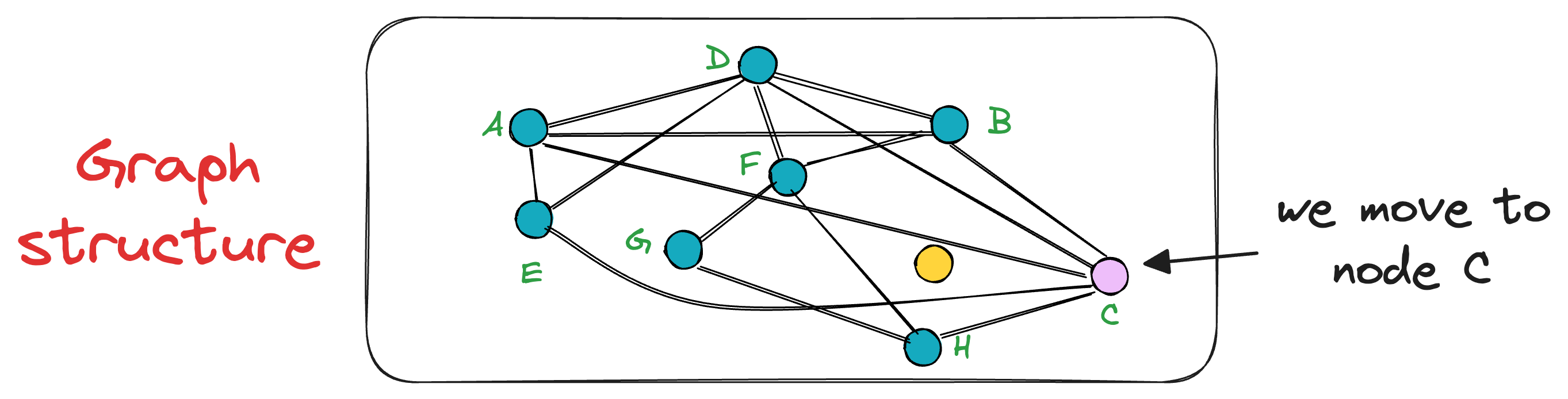
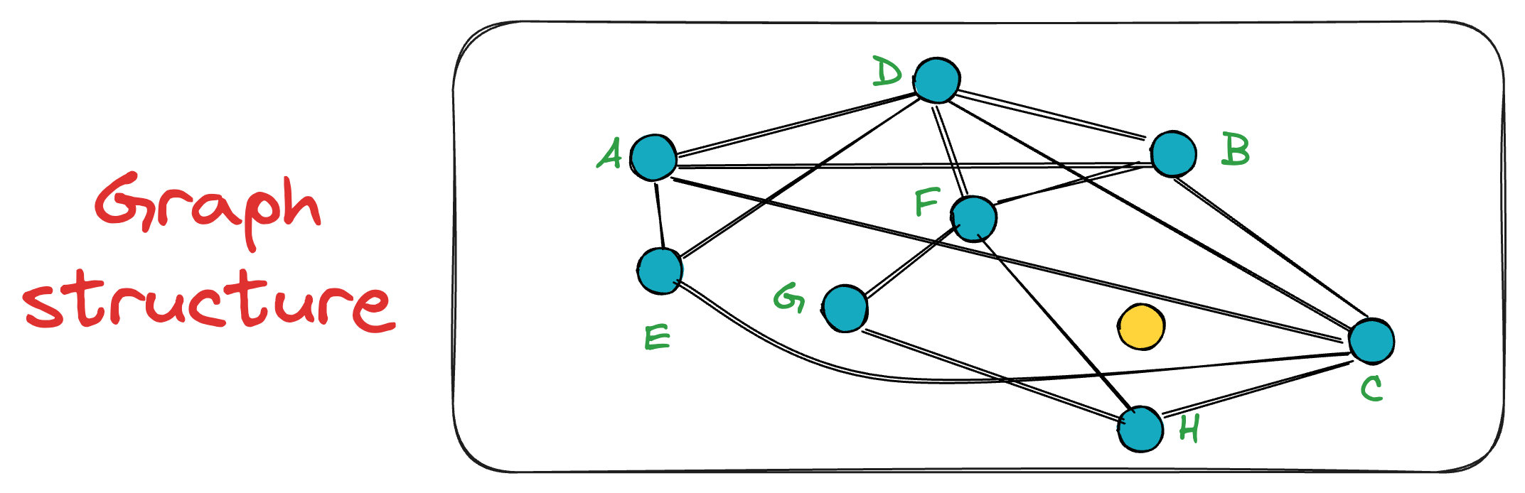
Next, the search moves toward the vertex with the least distance to the query vector.

The unevaluated neighbor of node C is only H, which turns out to be closer to the query vector, so we mode to node H now.

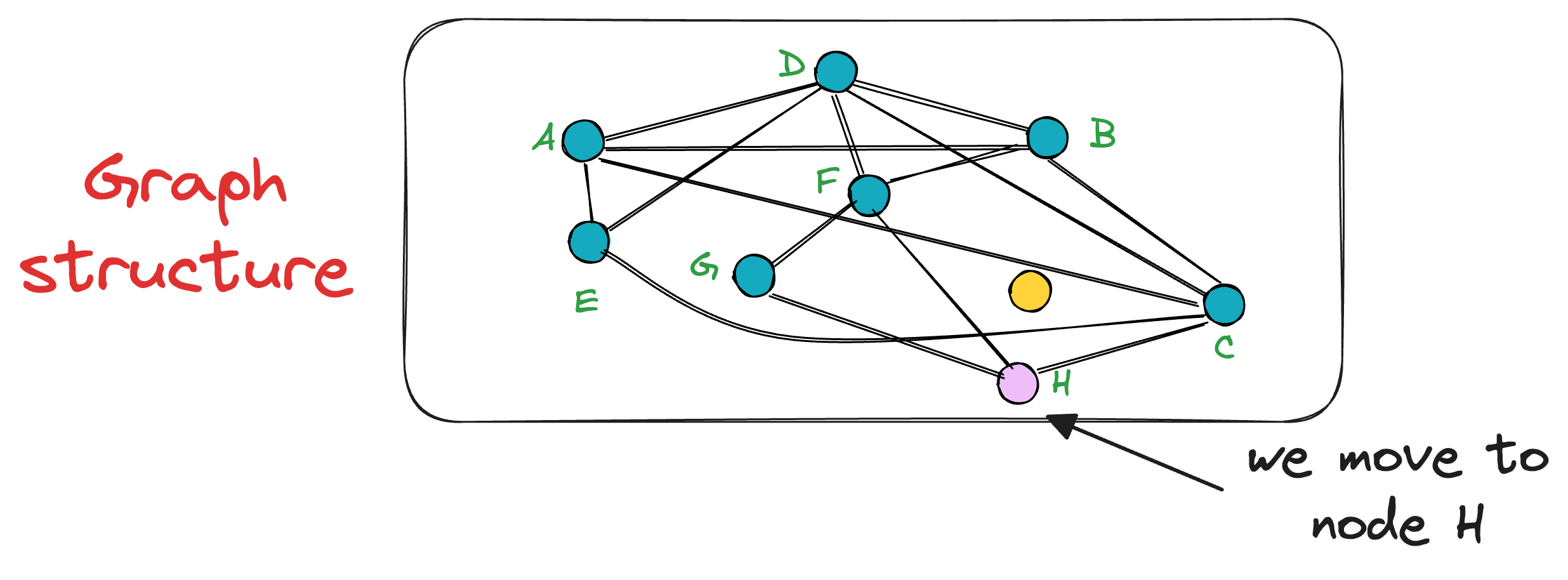
This process is repeated until no neighbor closer to the query vector can be found, which gives us the nearest neighbor in the graph for a query vector.

One thing I like about this search algorithm is how intuitive and easy to implement it is.

That said, the search is still approximate, and it is not guaranteed that we will always find the closest neighbor, and it may return highly suboptimal results.

For instance, consider this graph below, where node A is the entry point, and the yellow node is the vector we need the nearest neighbor for:

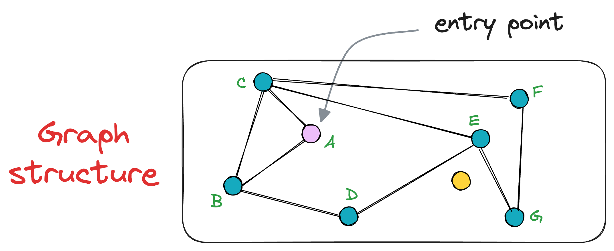
Following the above procedure of nearest neighbor search, we shall evaluate the neighbors of the node A, which are C and B.

It is clear that both nodes are further distant from the query vector than node A. Thus, the algorithm returns the node A as the final nearest neighbor.

To avoid such situations, it is recommended to repeat the search process with multiple entry points, which, of course, consumes more time.

→ Skip list data structure

While NSW is quite a promising and intuitive approach, another major issue is that we end up traversing the graph many times (or repeating the search multiple times) to arrive at an optimal approximate nearest neighbor node.

HNSW speeds up the search process by indexing the vector database into a more optimal graph structure, which is based on the idea of a skip list.

First, let me give you some details about the skip list data structure, as that is important here.

And to do this, let’s consider a pretty intuitive example that will make it pretty clear.

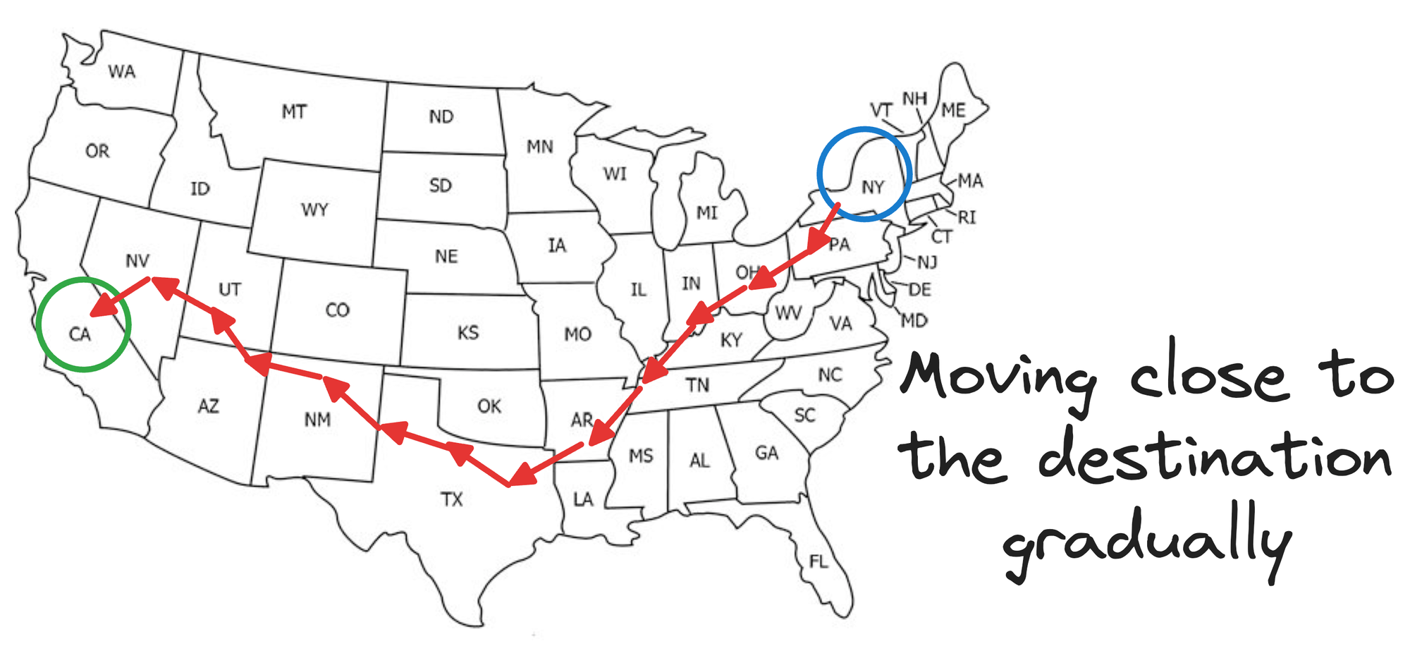
Say you wish to travel from New York to California.

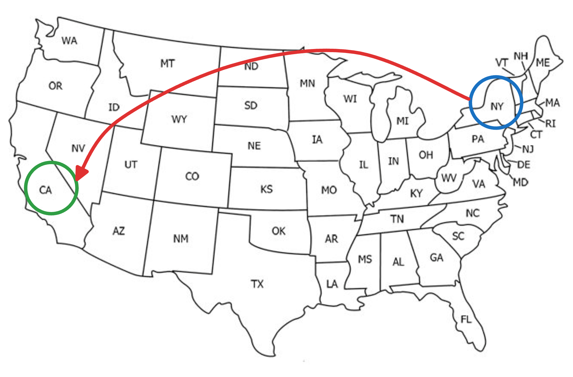
If we were following an NSW approach, this journey would be like traveling from one city to another, say, via an intercity taxi, which takes many hops, but gradually moves us closer to our destination, as shown below:

Is that optimal?

No right?

Now, think about it for a second.

How can you more optimally cover this route, or how would you more optimally cover this in real life?

If you are thinking of flights, you are thinking in the right direction.

Think of skip lists as a way to plan your trip using different modes of transportation, of which, some modes can travel larger distances in small hops.

So essentially, instead of hopping from one city to another, we could start by taking a flight from New York to a major city closer to California, say Denver.

This flight covers a longer distance in a single hop, analogous to skipping several vertices in the graph that we would have covered otherwise going from one city to another.

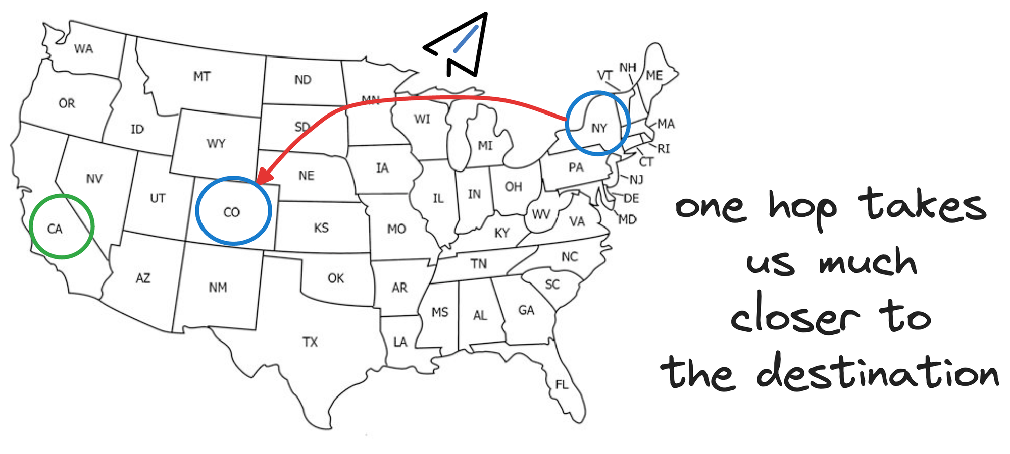
From Denver, we can take another faster mode of transport, which will involve fewer hops, like a train to reach California:

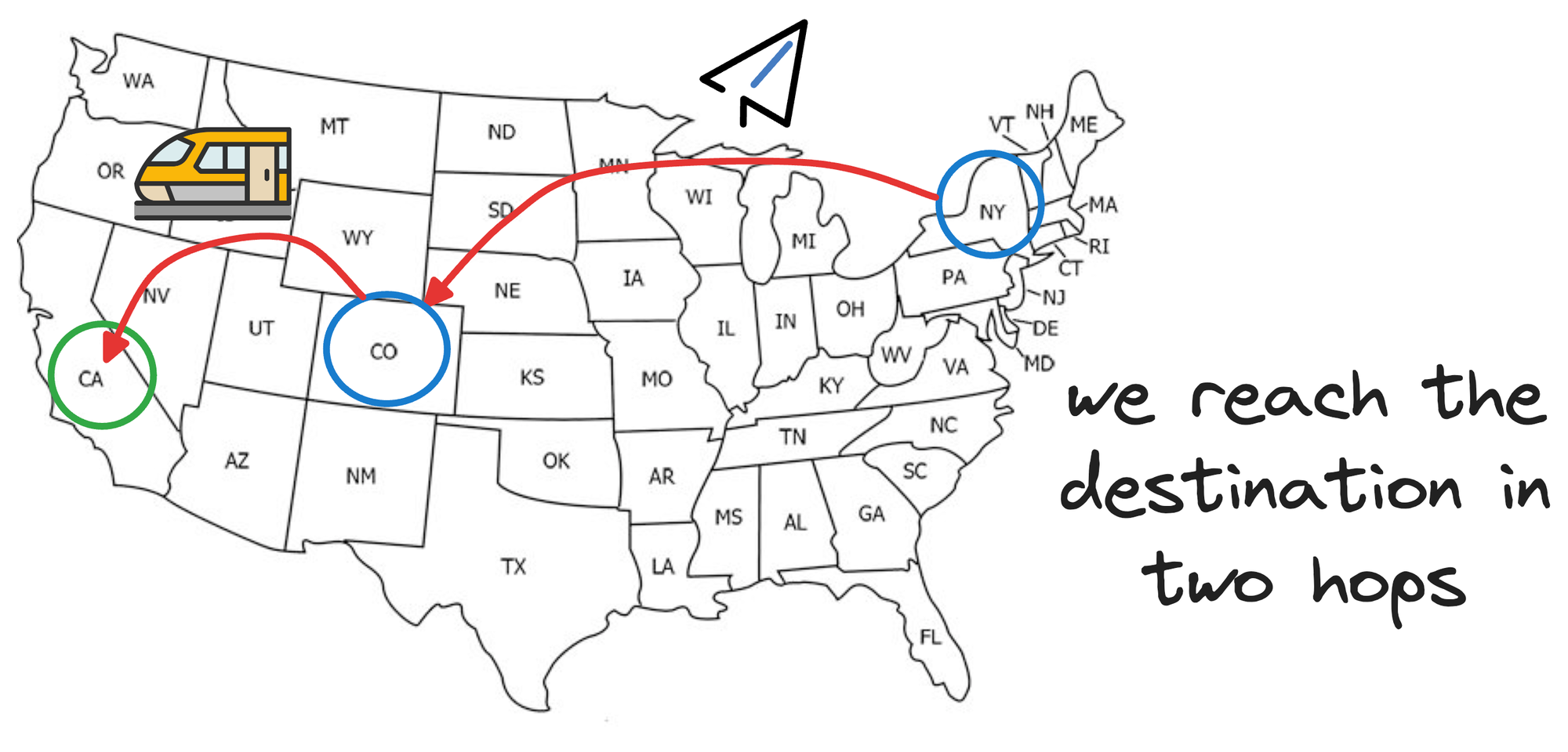
To add even more granularity, say, once we reach the train station in California, we wish to travel to some place within Los Angeles, California.

Now we need something that can take smaller hops, so a taxi is perfect here.

So what did we do here?

This combination of longer flights, a relatively shorter train trip, and a taxi to travel within the city allowed us to reach our destination in relatively very few stops.

This is precisely what skip lists do.

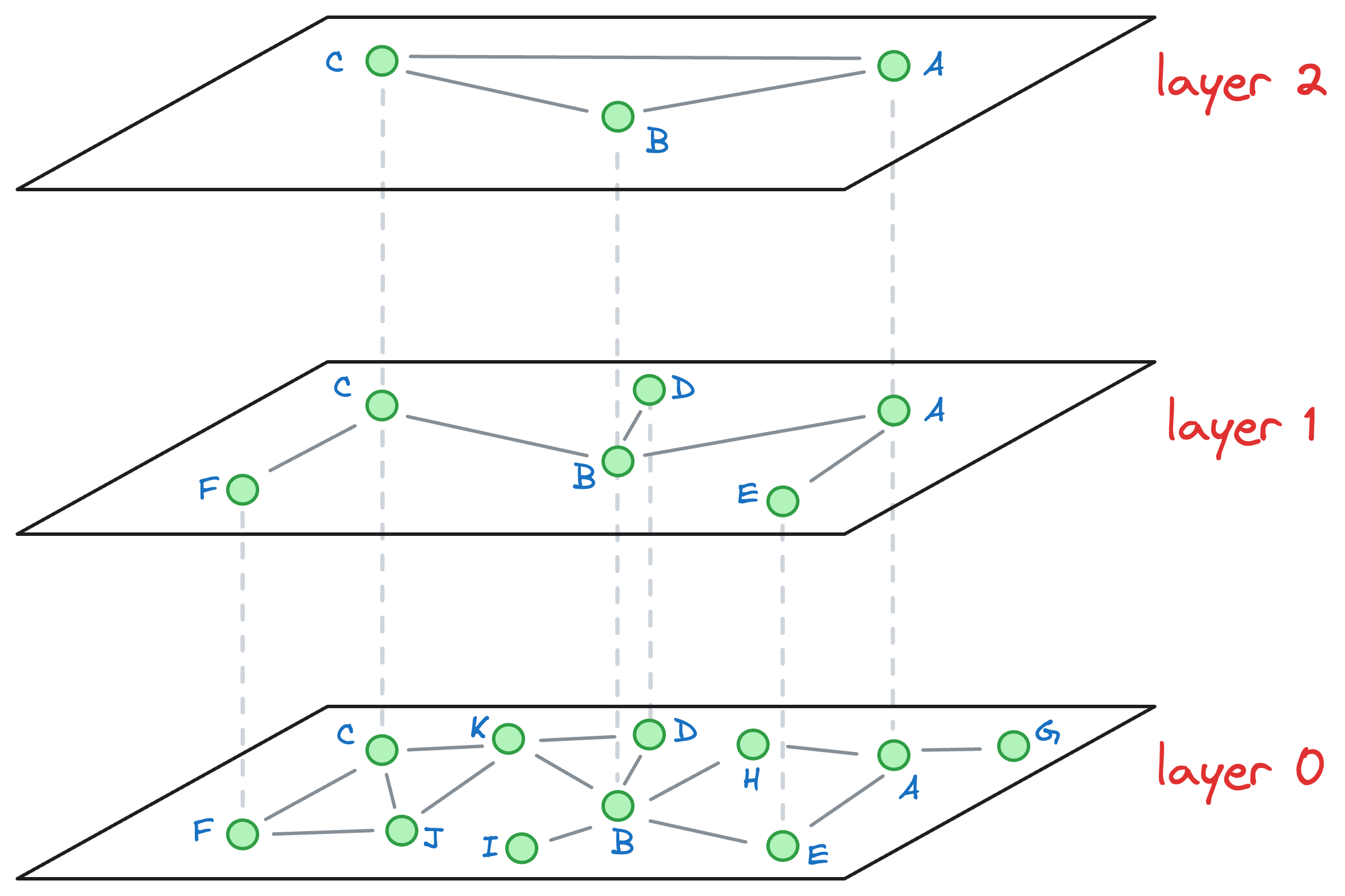
Skip lists are a data structure that allows for efficient searching of elements in a sorted list. They are similar to linked lists but with an added layer of "skip pointers" that allow faster traversal.

This is what linked lists look like:

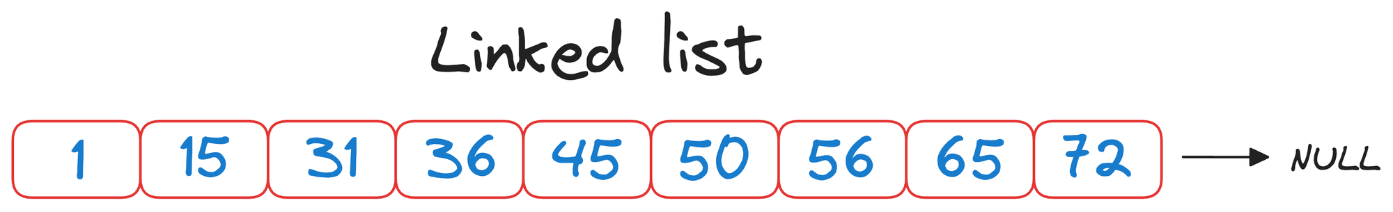
In a skip list, each element (or node) contains a value and a set of forward pointers that can "skip" over several elements in the list.

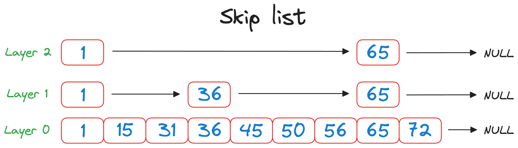
These forward pointers create multiple layers within the list (layer 0, layer 1, layer 2, in the above visual), with each level representing a different "skip distance."

• Top layer (layer 2) can be thought of as a flight that can travel longer distances in one hop.
• Middle layer (layer 1) can be thought of as a train that can travel relatively shorter distances than a flight in one hop.
• Bottom layer (layer 0) can be thought of as a taxi that can travel short distances in one hop.

The nodes that must be kept in each layer are decided using a probabilistic approach.

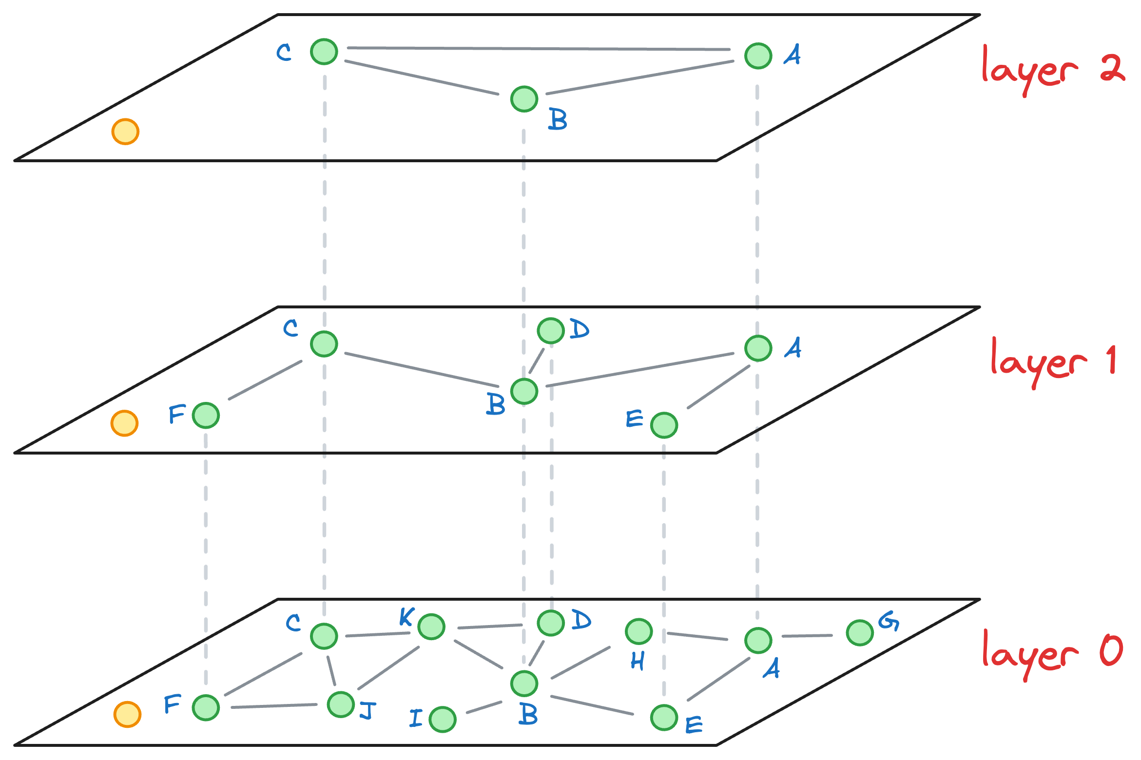
The basic idea is that nodes are included in higher layers with decreasing probability, resulting in fewer nodes at higher levels, while the bottom layer ALWAYS contains all nodes.

More specifically, before skip list construction, each node is randomly assigned an integer L, which indicates the maximum layer at which it can be present in the skip list data structure. This is done as follows:

• uniform(0,1) generates a random number between 0 and 1.
• floor() rounds the result down to the nearest integer.
• $C_{LM}$​ is a layer multiplier constant that adjusts the overlap between layers. Increasing this parameter leads to more overlap.

For instance, if a node has L=2, which means it must exist on layer 2, layer 1 and layer 0.

Also, say the layer multiplier ($C_{LM}$) was set to 0. This would mean that L=0 for all nodes:

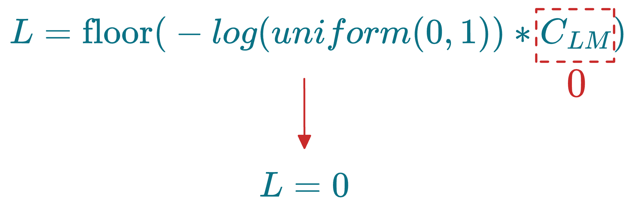
As discussed above, L indicates the maximum layer at which a node can be present in the skip list data structure. If L=0 for all nodes, this means that the skip list will only have one layer.

Increasing this parameter leads to more overlap between layers and more layers, as shown in the plots below:

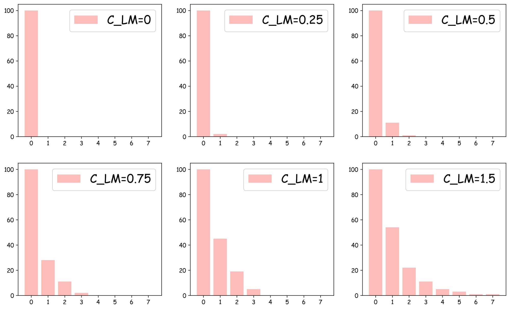
As depicted above:

• With $C_{LM}=0$, the skip list can only have layer 0, which is similar to the NSW search.
• With $C_{LM}=0.25$, we get one more layer, which has around 6-7 nodes.
• With $C_{LM}=1$, we get four layers.
• In all cases, layer 0 always has all nodes.

The objective is to decide an optimal value for $C_{LM}$ because we do not want to have too many layers and so much overlap, while, at the same time, also not having only one layer (when $C_{LM}=0), which would result in no speedup improvement.

Now, let me explain how skip lists speedup the search process.

Let’s say we want to find the element 50 in this list.

If we were using the typical linked list, we would have started from the first element (HEAD), and scanned each node one by one to see and check if it matches the query or not (50).

See how a skip list helps us optimize this search process.

We begin from the top layer (layer 2) and check the value corresponding to the next node in the same layer, which is 65.

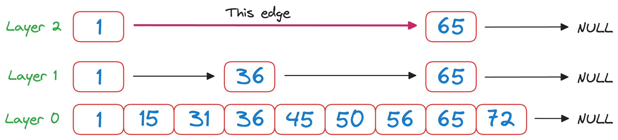
As 65>50 and it is a unidirectional linked list, we must go down one level.

In layer 1, we check the value corresponding to the next node in the same layer, which is 36.

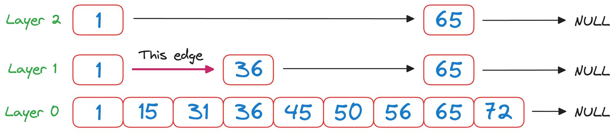
As 50>36 and it is wise to move to the node corresponding to the value 36.

Now again in layer 1, we check the value corresponding to the next node in the same layer, which is 65.

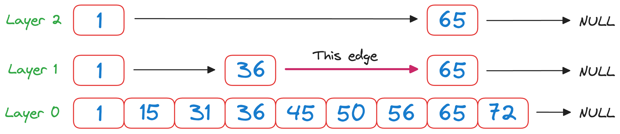
Again, as 65>50 and it is a unidirectional linked list, we must go down one level.

We reach layer 0, which can be traversed the way we usually would.

Had we traversed the linked list without building a skip list, we would have taken 5 hops:

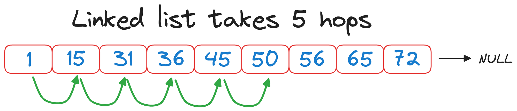
But with a skip list, we completed the same search in 3 hops instead:

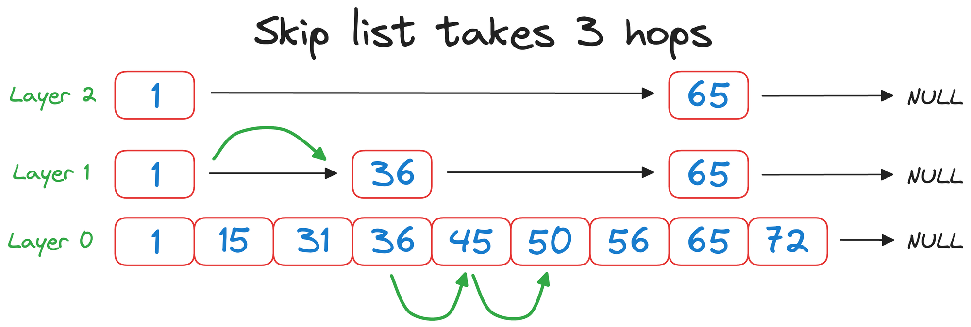
That was pretty simple and elegant, wasn't it?

While reducing the number of hops from 5 to 3 might not sound like a big improvement, but it is important to note that typical vector databases have millions of nodes.

Thus, such improvements scale pretty quickly to provide run-time benefits.

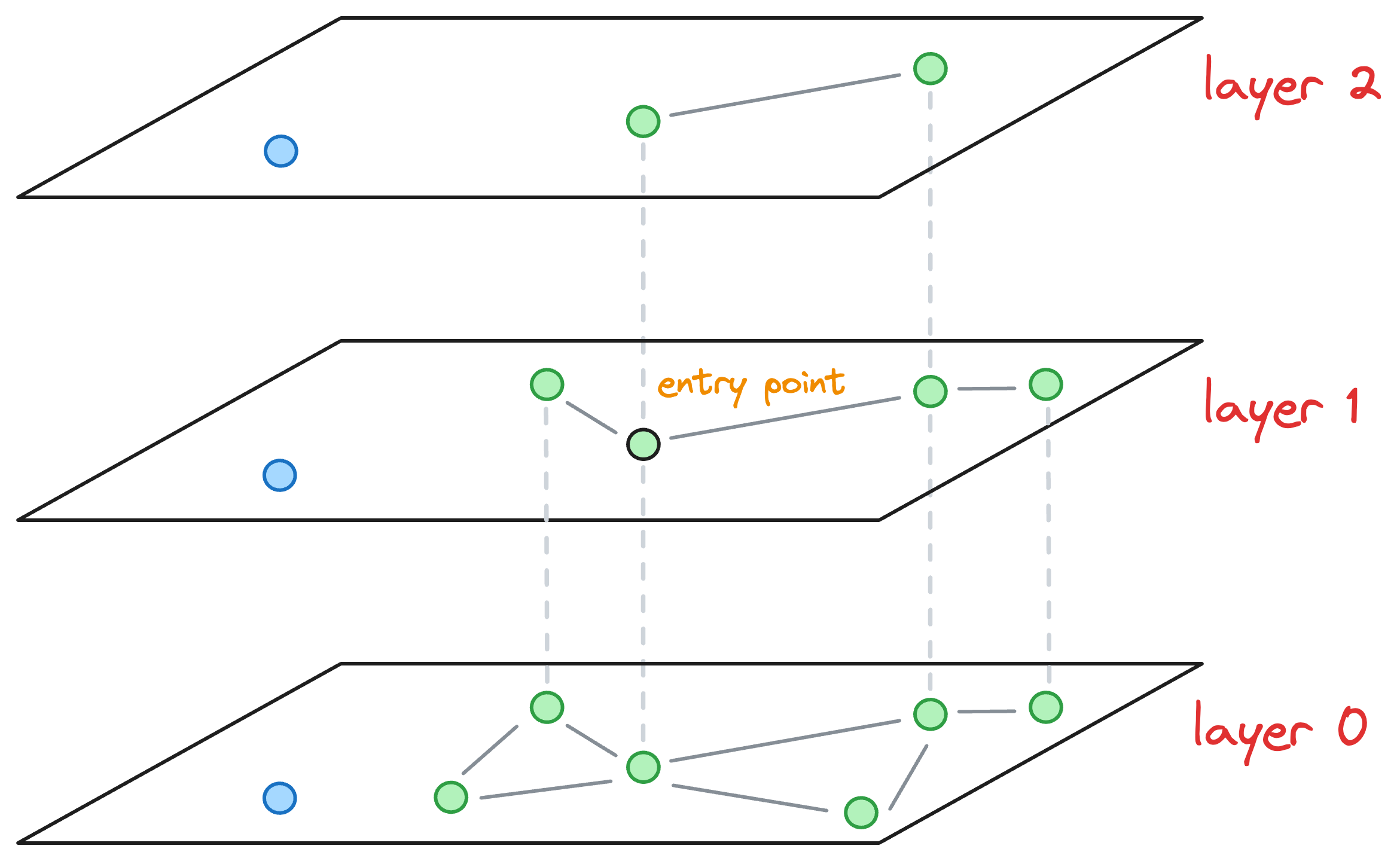
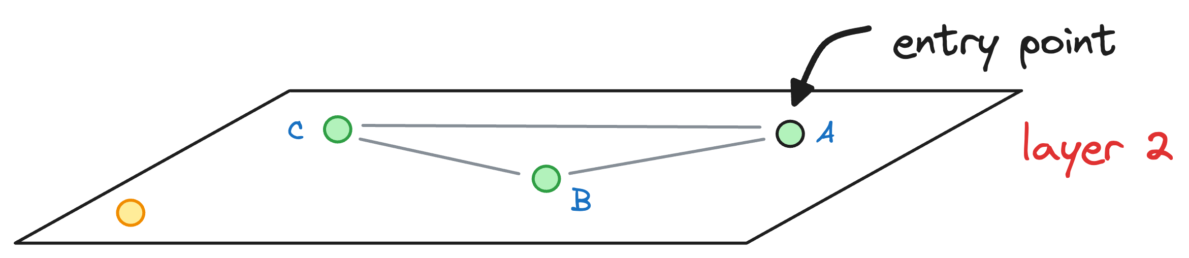
→ Graph construction in HNSW

Now that we understand how skip lists work, understanding the graph construction process of Hierarchical Navigable Small World is also pretty straightforward.

Consider that this is our current graph structure:

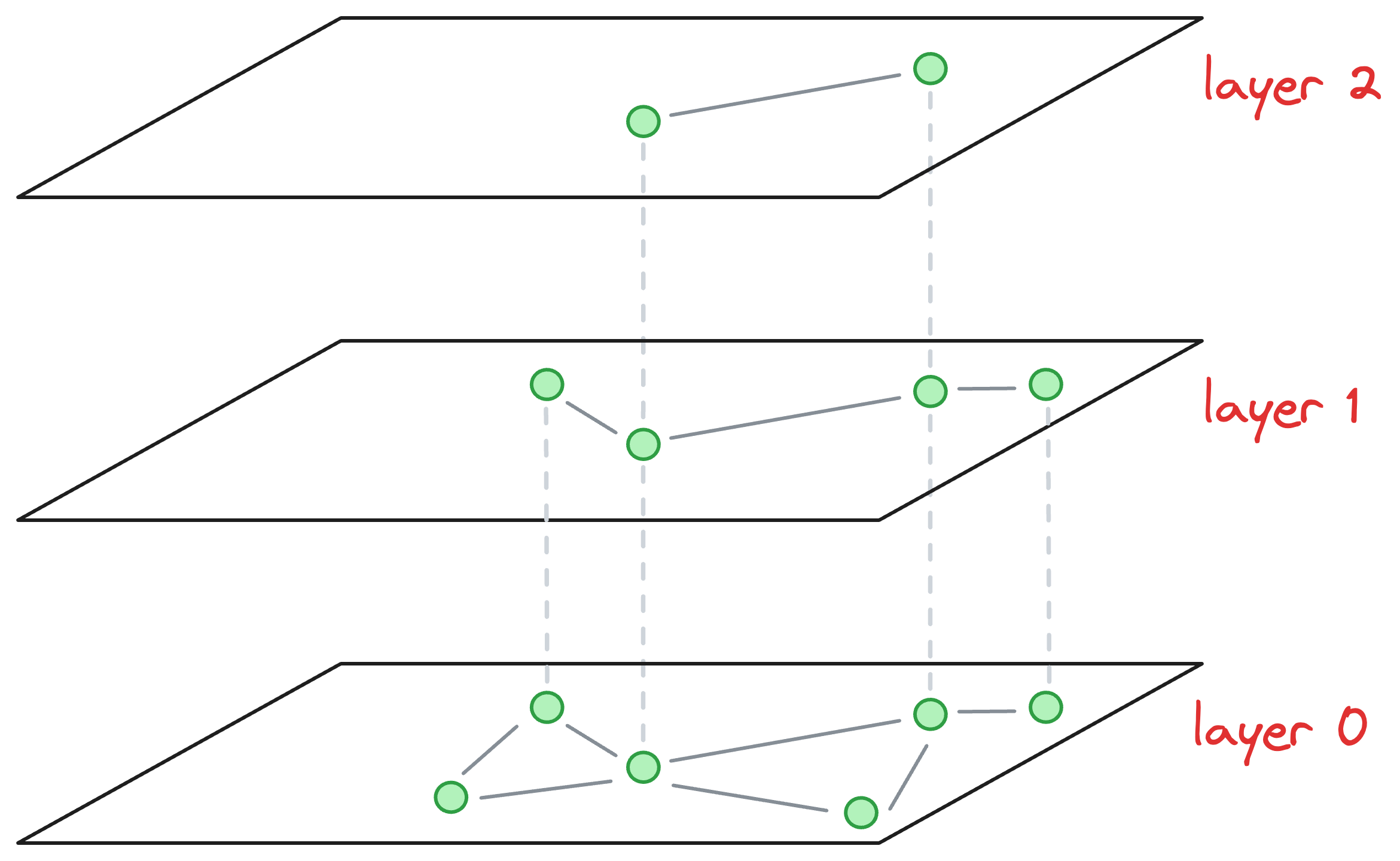
I understand we are starting in the middle of the construction process, but just bear with me for a while, as it will clear everything up.

Essentially, the above graph has three layers in total, and it is in the middle of construction. Also, as we go up, the number of nodes decreases, which is what happens ideally in skip lists.

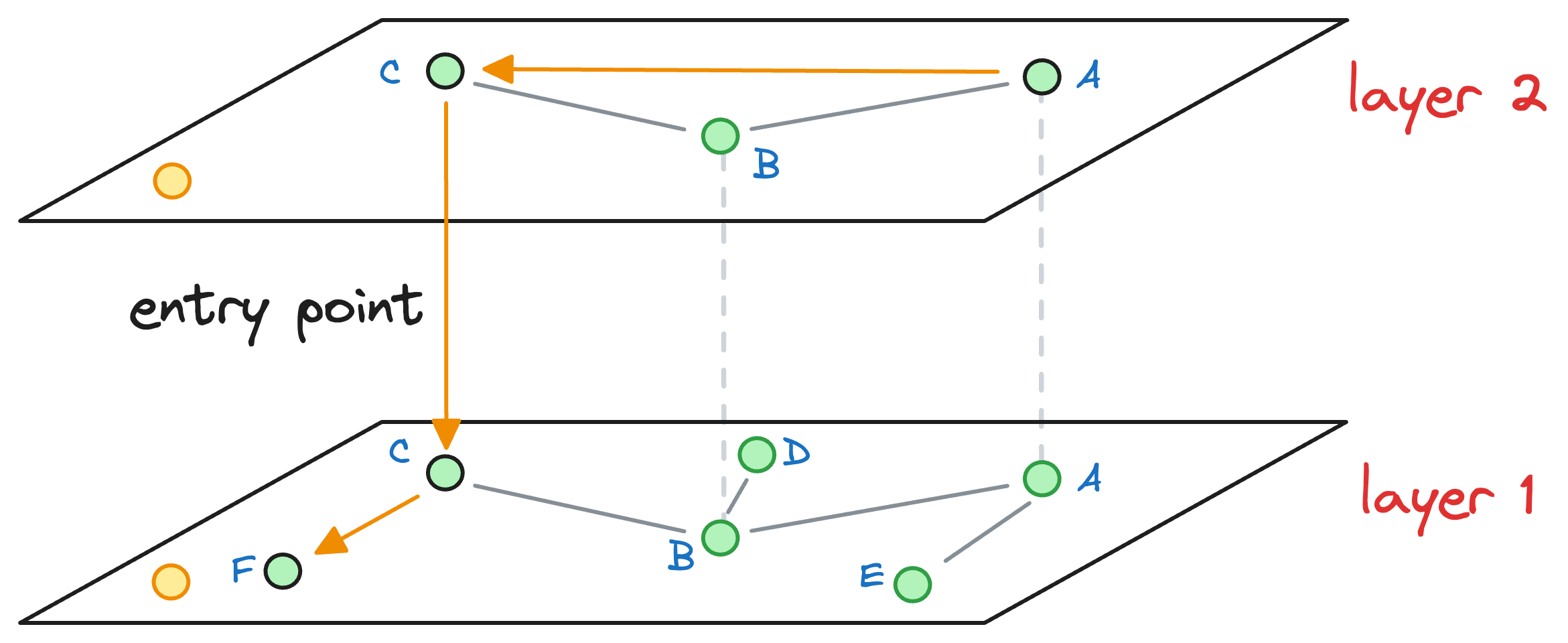
Now, let’s say we wish to insert a new node (blue node in the image below), and its max level (determined by the probability distribution) is L=1. This means that this node will be present on layer 1 and layer 0.

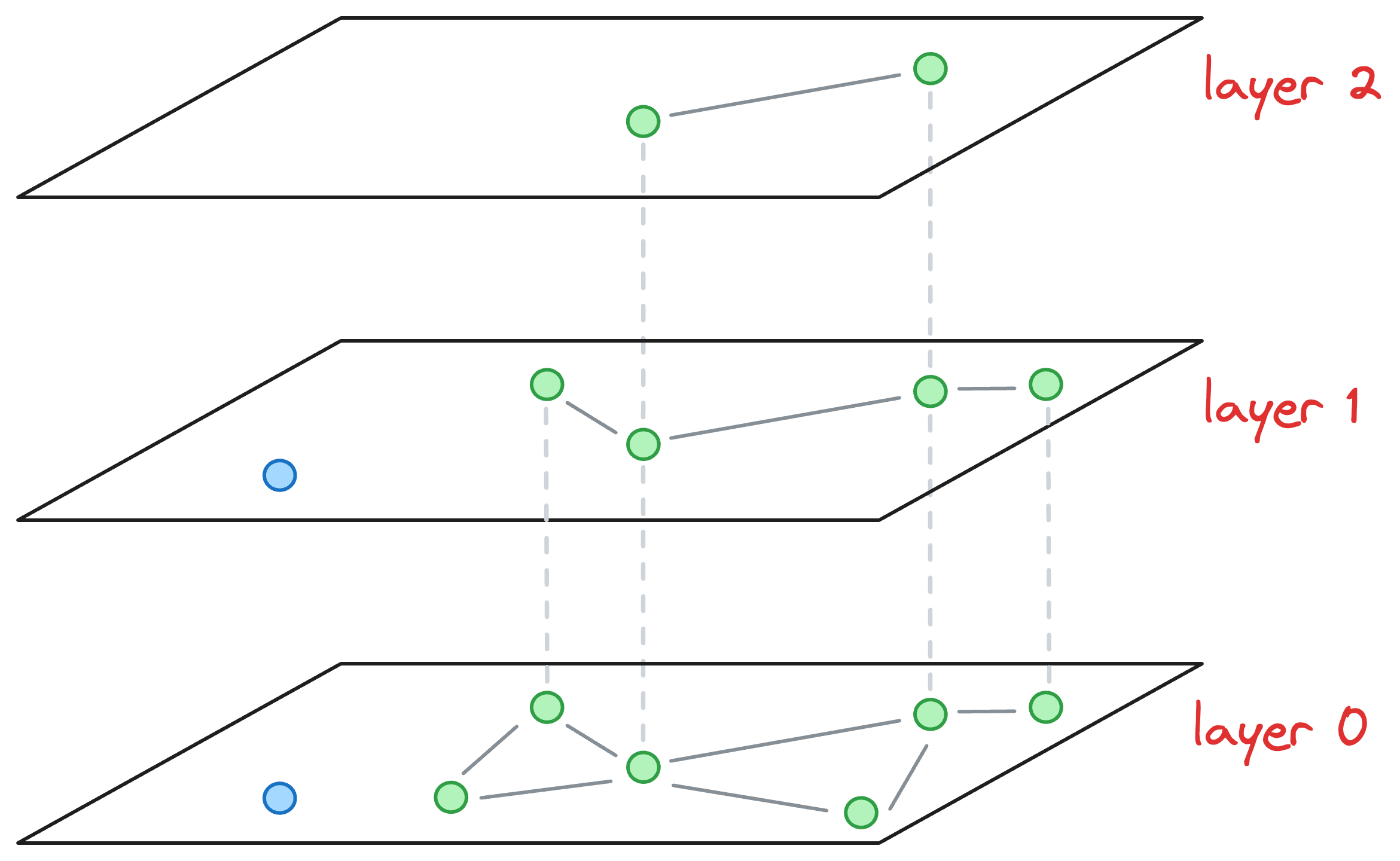
Now, our objective is to connect this new node to other nodes in the graph on layer 0 and layer 1.

This is how we do it:

• We start from the topmost layer (layer 2) and select an entry point for this new node randomly:

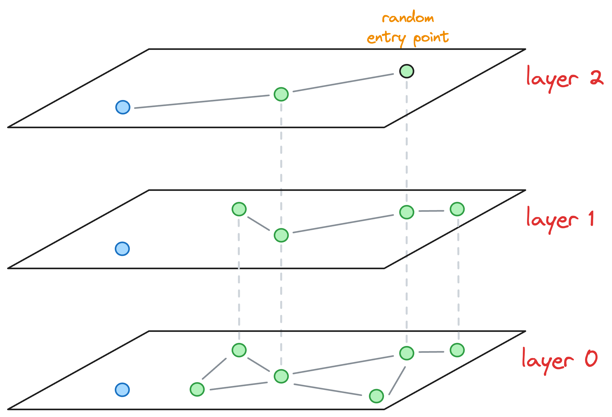
• We explore the neighbors of this entry point and select the one that is nearest to the new node to be inserted.

• The nearest neighbor found for the blue node becomes the entry point for the next layer. Thus, we move to the corresponding node of the nearest neighbor in the next layer (layer 1):

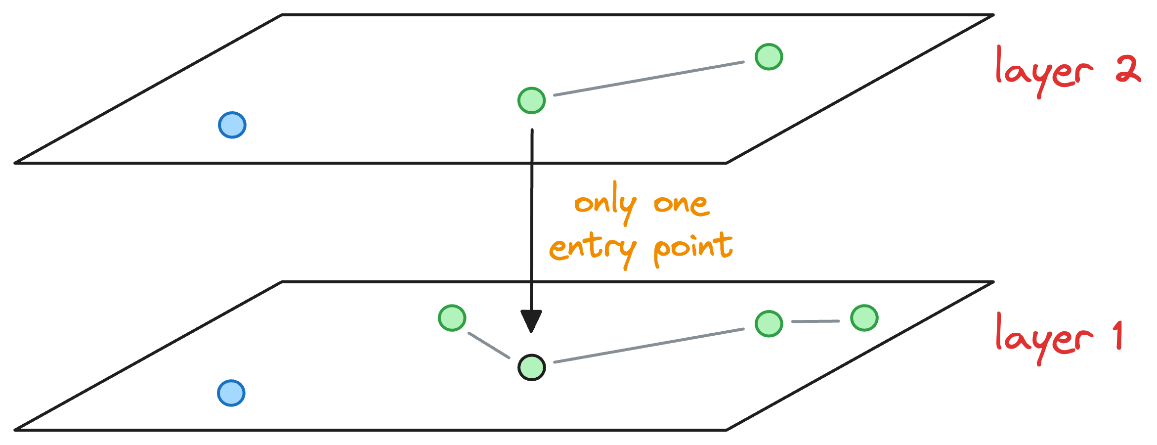
• With that, we have arrived at the layer where this blue node must be inserted.

Here, note that had there still been more layers, we would have repeated the above process of finding the nearest neighbor of the entry point and moving one layer down until we had arrived at the layer of interest.

For instance, imagine that the max level value for this node was L=0. Thus, the blue node would have only existed on the bottom-most layer.

After moving the layer 1 (as shown in the figure above), we haven't arrived at the layer of interest yet.

So we explore the neighborhood of the entry point in layer 1 and find the nearest neighbor of the blue point again.

Now, the nearest neighbors found on layer 1 becomes our entry point for layer 0.

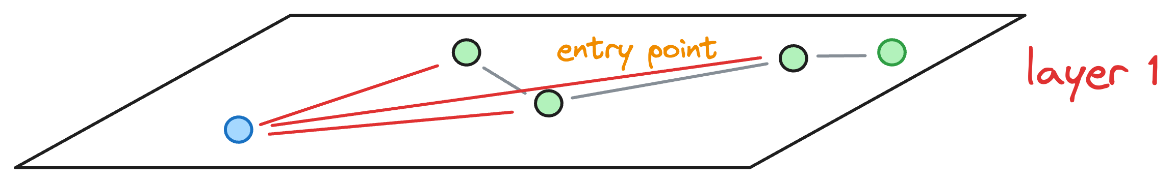
Coming back to the situation where the max level value was L=1. We are currently at layer 1, where the entry point is marked in the image below, and we must insert the blue node on this layer:

To insert a node, here’s what we do:

• Explore the neighbors of the entry point in the current layer and connect the new node to the top K nearest neighbors. To determine the top K neighbors, a total of efConstruction (a hyperparameter) neighbors are greedily explored in this step. For instance, if K=2, then in the above diagram, we connect the blue node to the following nodes:

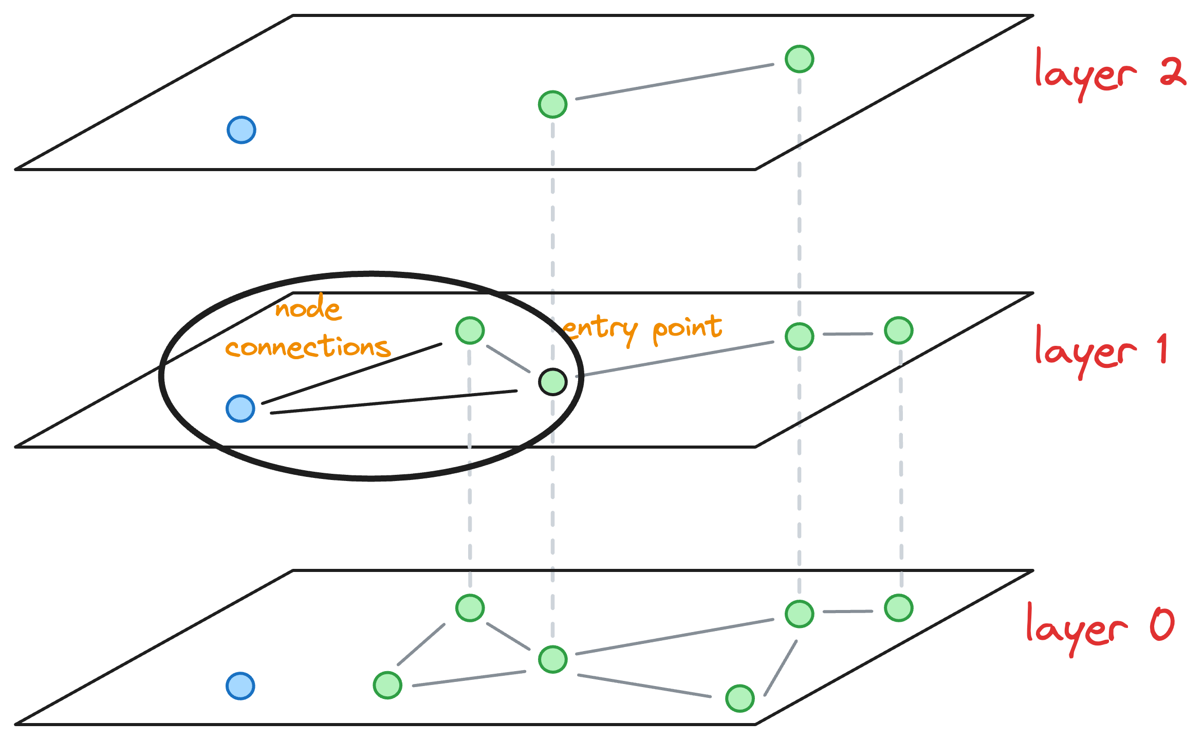
However, to determine these top K=2 nodes, we may have explored, say efConstruction=3 neighbors instead (the purpose of doing this will become clear shortly), as shown below:

Now, we must insert the blue node at a layer that is below the max layer value L of the blue node.

In such a case, we don’t keep just one entry point to the next layer, like we did earlier, as shown below:

However, all efConstruction nodes explored in the above layer are considered as an entry point for the next layer.

Once we enter the next layer, The process is repeated, wherein, we connect the blue node to the top K neighbors by exploring all efConstruction entry nodes.

The layer-by-layer insertion process ends when the new node gets connected to nodes at level 0.

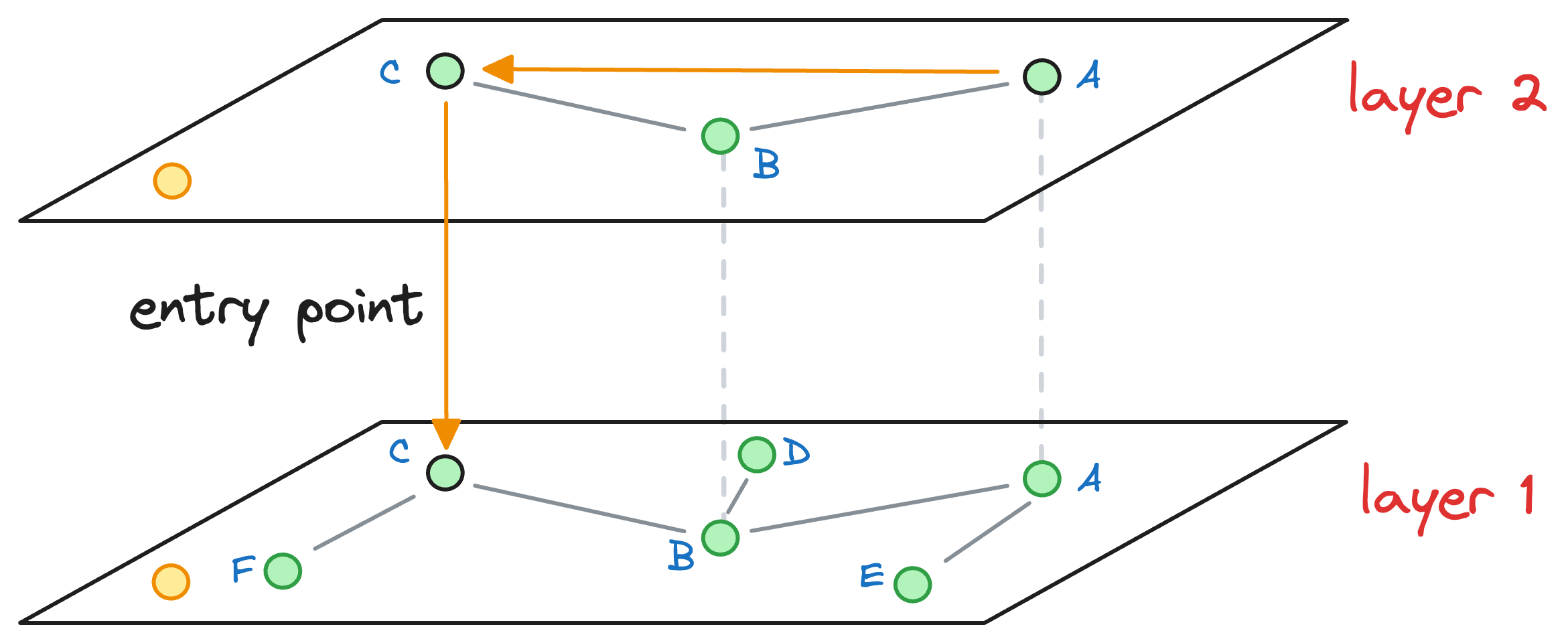
→ Search in HNSW

Consider that after all the nodes have been inserted, we get the following graph:

Let’s understand how the approximate nearest neighbor search would work.

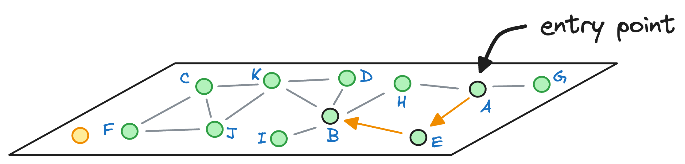
Say we want to find the nearest neighbor of the yellow vector in the image below:

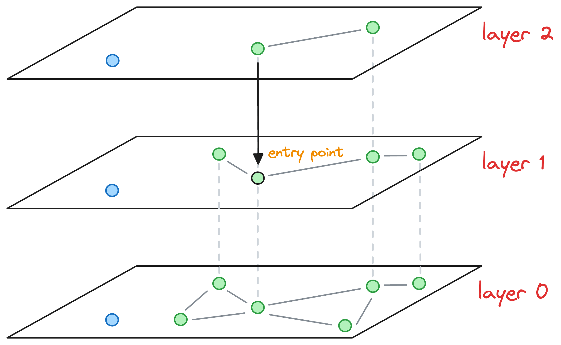
We begin our search with an entry point in the top layer (layer 2):

We explore the connected neighbors of A and see which is closest to the yellow node. In this layer, it is C.

The algorithm greedily explores the neighborhood of vertices in a layer. We consistently move towards the query vector during this process.

When no closer node can be found in a layer that is closer to the query vector, we move to the next layer while considering the nearest neighbor (C, in this case) as an entry point to the next layer:

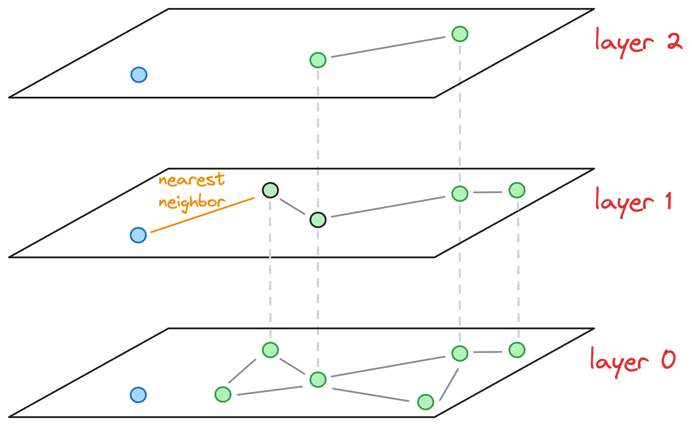
The process of neighborhood exploration is repeated again.

We explore the neighbors of C and greedily move to that specific neighbor which is closest to the query vector:

Again, as no node exists in layer 1 that is closer to the query vector, we move to the next layer while considering the nearest neighbor (F, in this case) as an entry point to the next layer.

But this time, we have reached layer 0. Thus, an approximate nearest neighbor will be returned in this case.

When we move to layer 0, and start exploring its neighborhood, we notice that it has no neighbors that are closer to the query vector:

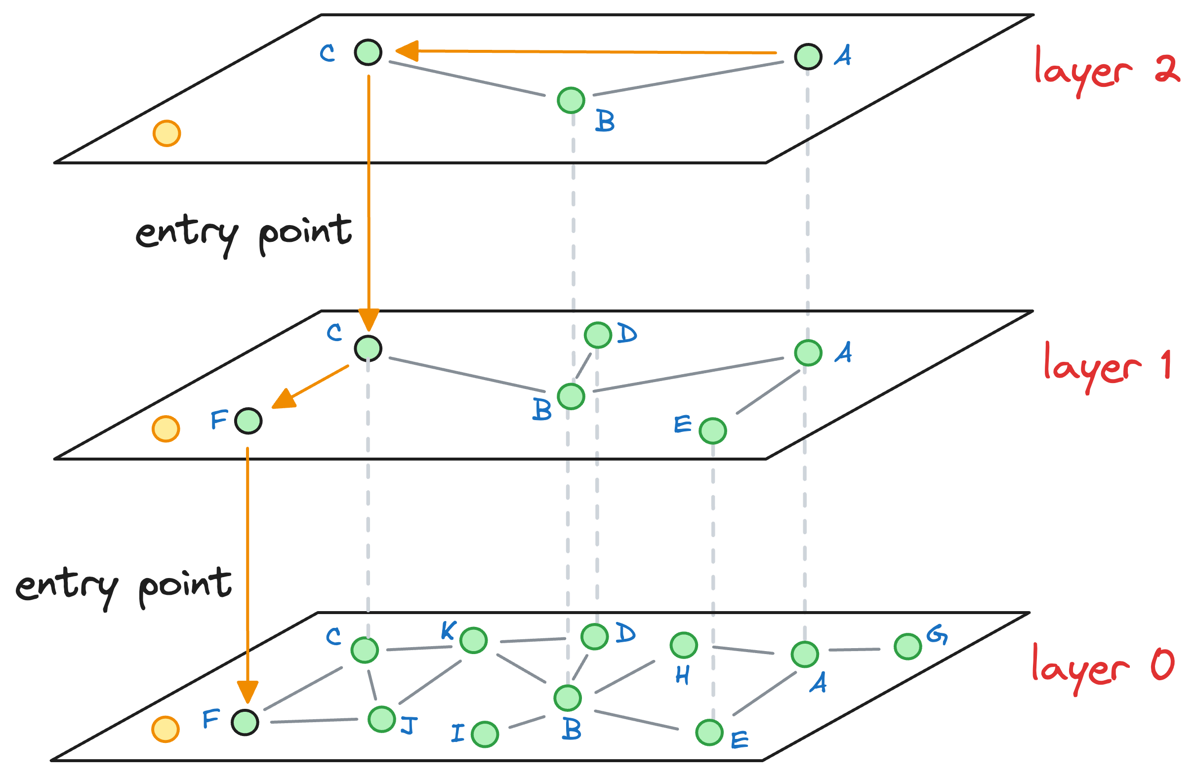
Thus, the vector corresponding to node F is returned as an approximate nearest neighbor, which, coincidentally, also happens to be the true nearest neighbor.

→ HNSW vs NSW

In the above search process, it only took 2 hops (descending is not a hop) to return the nearest neighbor to the query vector.

Let’s see how many hops it would have taken us to find the nearest neighbor with NSW. For simplicity, let’s consider that the graph constructed by NSW is the one represented by layer 0 of the HNSW graph:

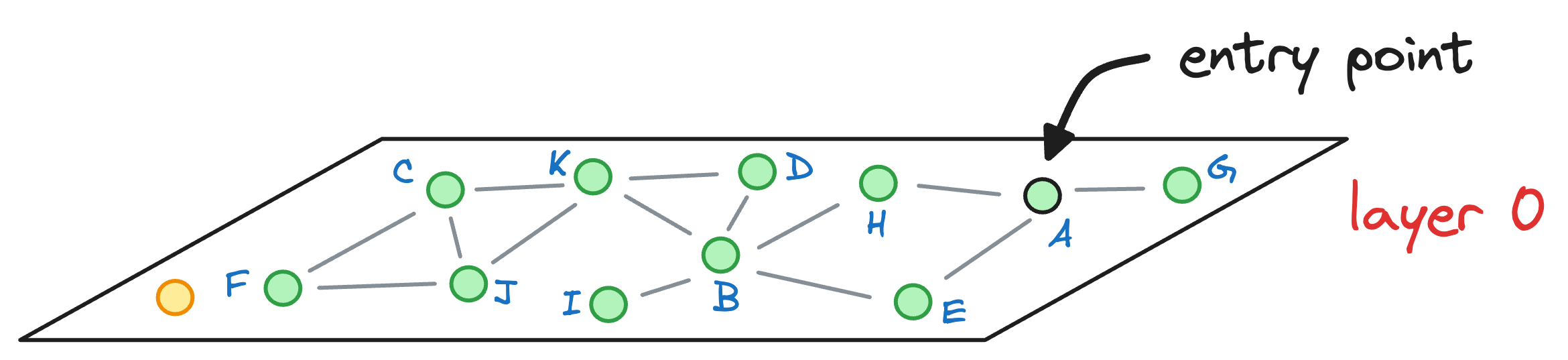
We started with the node A as the entry point earlier, so let’s consider the same here as well.

We begin with the node A, explore its neighbors, and move to the node E as that is the closest to the query vector:

From node E, we move to node B, which is closer to the query vector than the node E.

Next, we explore the neighbors of node B, and notice that node I is the closest to the query vector, so we hop onto that node now:

As node I cannot find any other node that it is connected to that is closer than itself, the algorithm returns node I as the nearest neighbor.

What happened there?

Not only did the algorithm take more hops (3) to return a nearest neighbor, but it also returned a less optimal nearest neighbor.

HNSW, on the other hand, took fewer hops and returned a more accurate and optimal nearest neighbor.

Perfect!

With that, you have learned five pretty common indexing strategies to index vectors in a vector database for efficient search.

Using Vector Databases in LLMs

At this point, one interesting thing to learn is how exactly do Large Language Models (LLMs) take advantage of Vector Databases.

In my experience, the biggest conundrum many people face is the following:

Once we have trained our LLM, it will have some model weights for text generation. Where do vector databases fit in here?

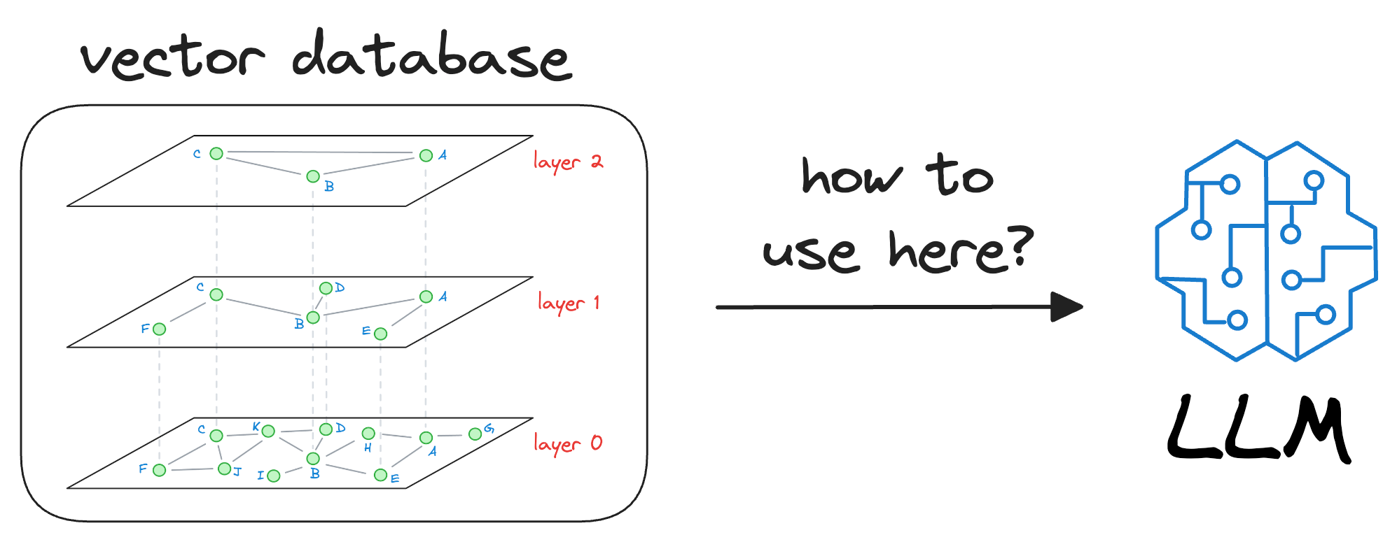
And it is a pretty genuine query, in my opinion.

Let me explain how vector databases help LLMs be more accurate and reliable in what they produce.

To begin, we must understand that an LLM is deployed after learning from a static version of the corpus it was fed during training.

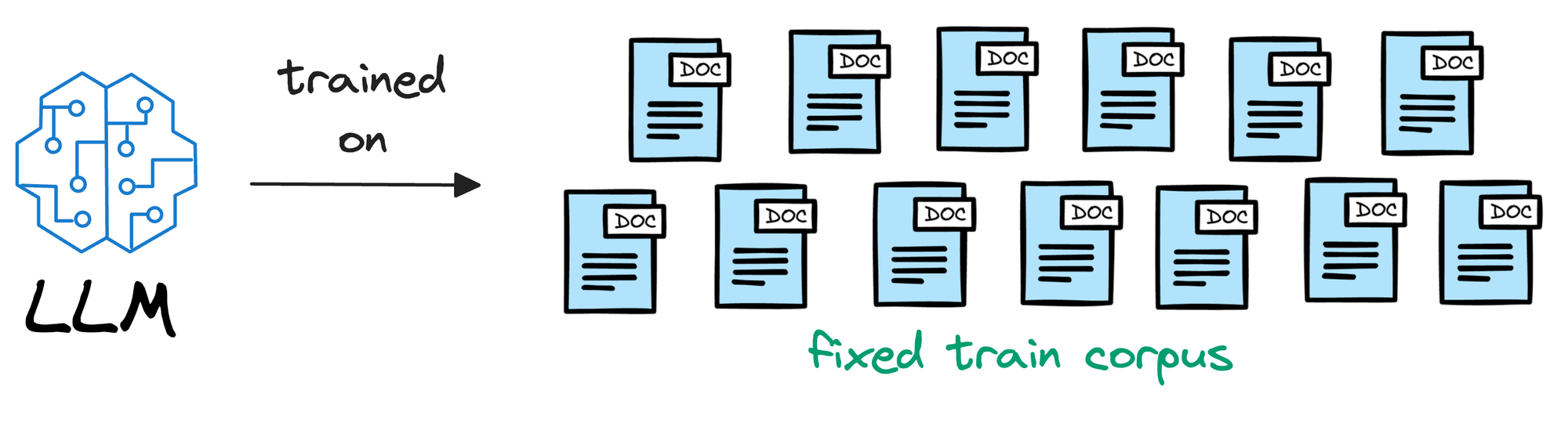
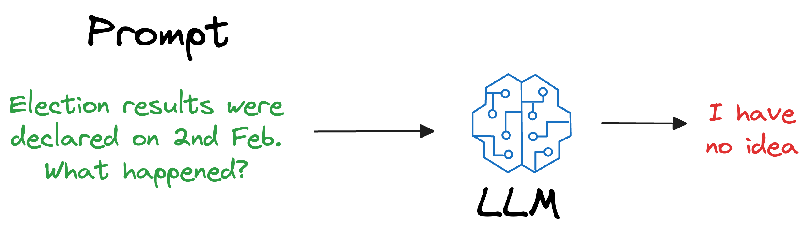
For instance, if the model was deployed after considering the data until 31st Jan 2024, and we use it, say, a week after training, it will have no clue about what happened in those days.

Repeatedly training a new model (or adapting the latest version) every single day on new data is impractical and cost-ineffective. In fact, LLMs can take weeks to train.

Also, what if we open-sourced the LLM and someone else wants to use it on their privately held dataset, which, of course, was not shown during training?

As expected, the LLM will have no clue about it.

But if you think about it, is it really our objective to train an LLM to know every single thing in the world?

A BIGGG NOOOO!

That’s not our objective.

Instead, it is more about helping the LLM learn the overall structure of the language, and how to understand and generate it.

So, once we have trained this model on a ridiculously large enough training corpus, it can be expected that the model will have a decent level of language understanding and generation capabilities.

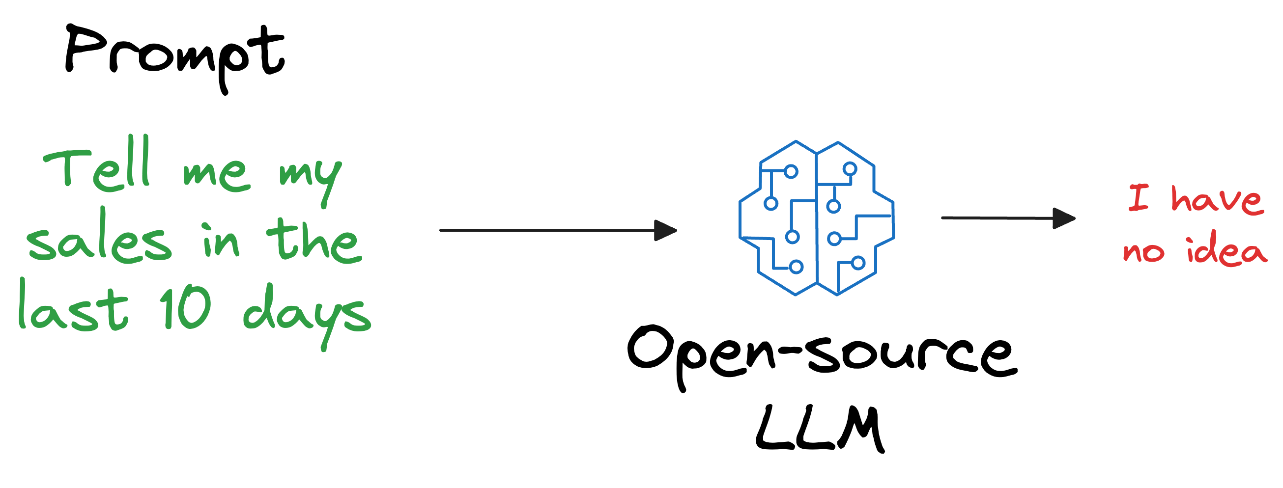
Thus, if we could figure out a way for LLMs to look up new information they were not trained on and use it in text generation (without training the model again), that would be great!

One way could be to provide that information in the prompt itself.

In other words, if training or fine-tuning the model isn’t desired, we can provide all the necessary details in the prompt given to the LLM.

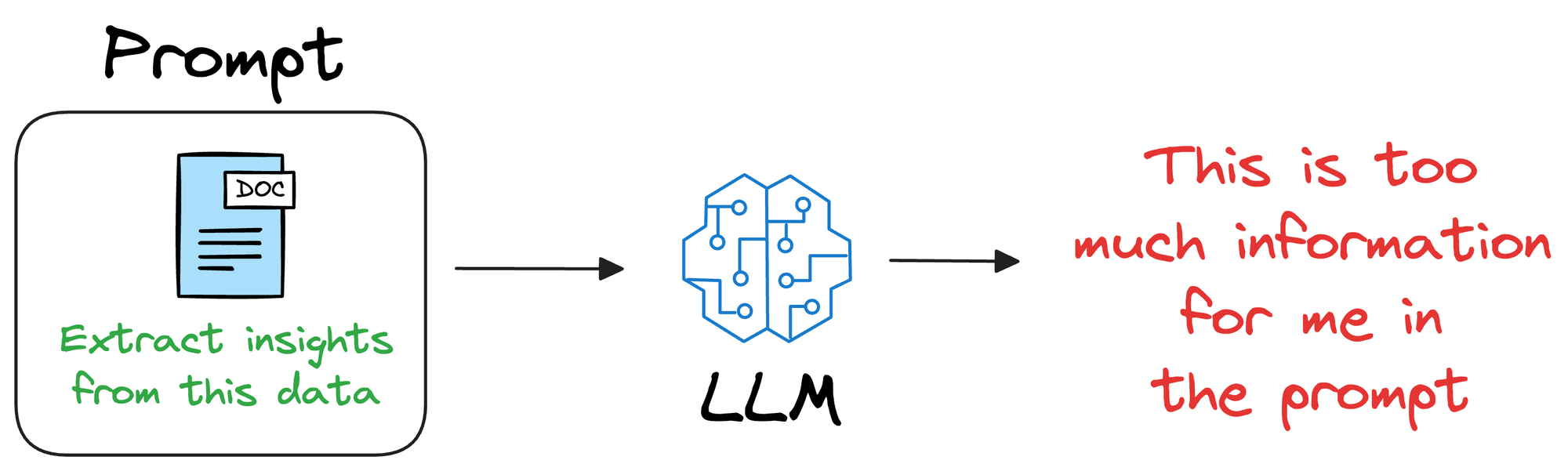
Unfortunately, this will only work for a small amount of information.

This is because LLMs are auto-regressive models.

Thus, as the LLM considers previous words, they have a token limit that they practically can not exceed in their prompts.

Overall, this approach of providing everything in the prompt is not that promising because it limits the utility to a few thousand tokens, whereas in real life, additional information can have millions of tokens.

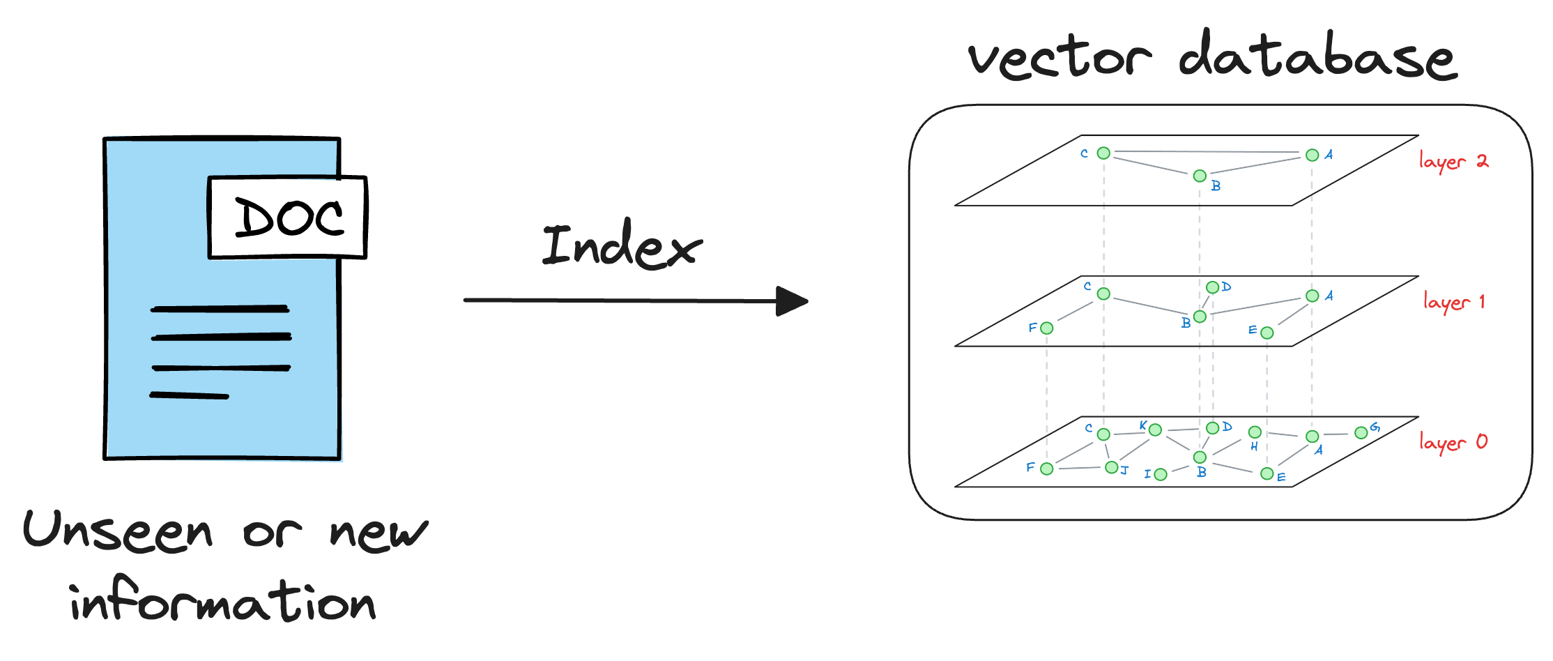
This is where vector databases help.

Instead of retraining the LLM every time new data emerges or changes, we can leverage vector databases to update the model's understanding of the world dynamically.

How?

It’s simple.

As discussed earlier in the article, vector databases help us store information in the form of vectors, where each vector captures semantic information about the piece of text being encoded.

Thus, we can maintain our available information in a vector database by encoding it into vectors using an embedding model.

When the LLM needs to access this information, it can query the vector database using a similarity search with the prompt vector.

More specifically, the similarity search will try to find contents in the vector database that are similar to the input query vector.

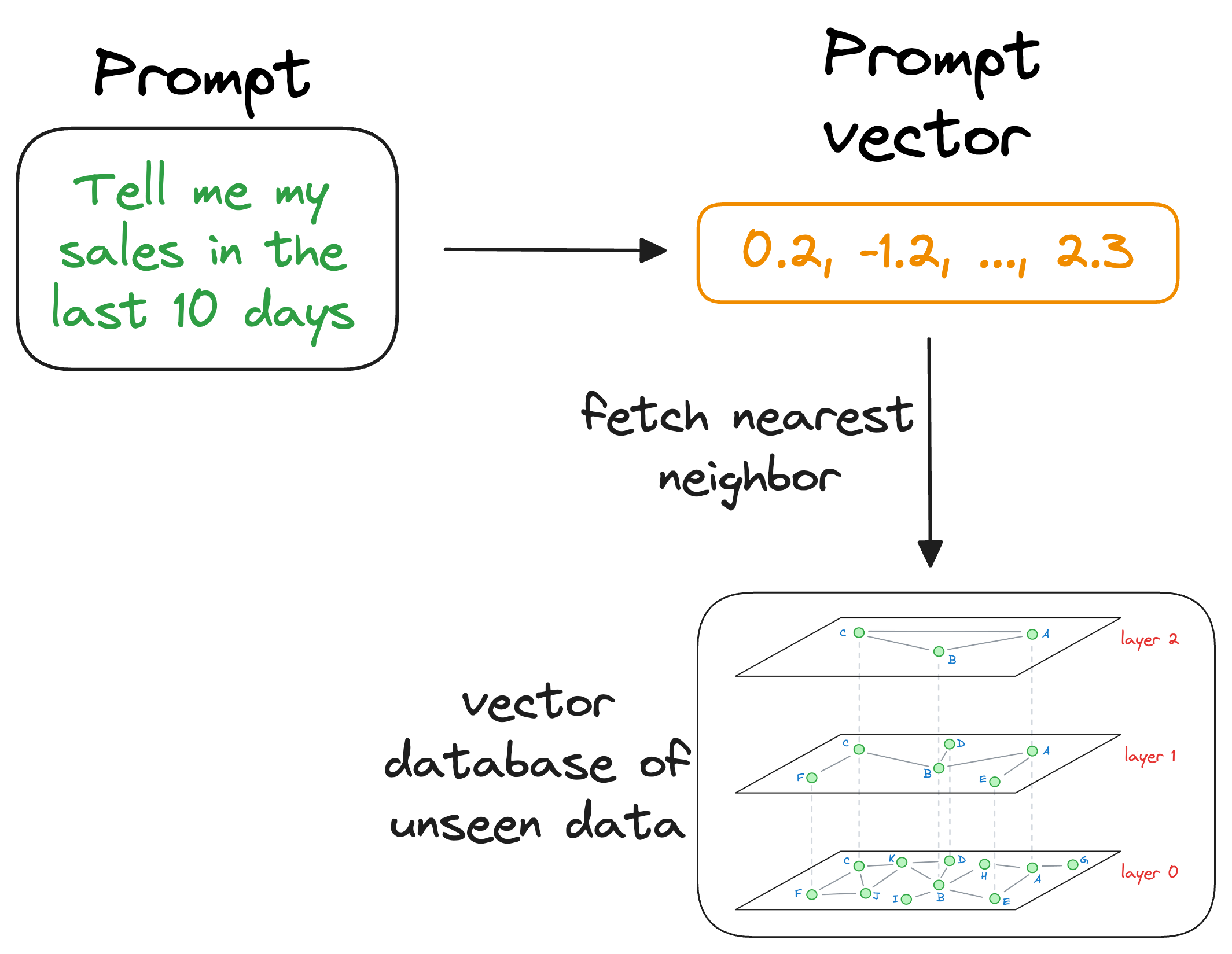
This is where indexing becomes important because our vector database can possibly have millions of vectors.

Theoretically, we can compare the input vector to every vector in the vector database.

But for practical utility, we must find the nearest neighbor as quickly as possible.

That is why indexing techniques, which we discussed earlier, become so important. They help us find the approximate nearest neighbor in almost real-time.

Moving on, once the approximate nearest neighbor gets retrieved, we gather the context from which those specific vectors were generated. This is possible because a vector database not only stores vectors but also the raw data that generated those vectors.

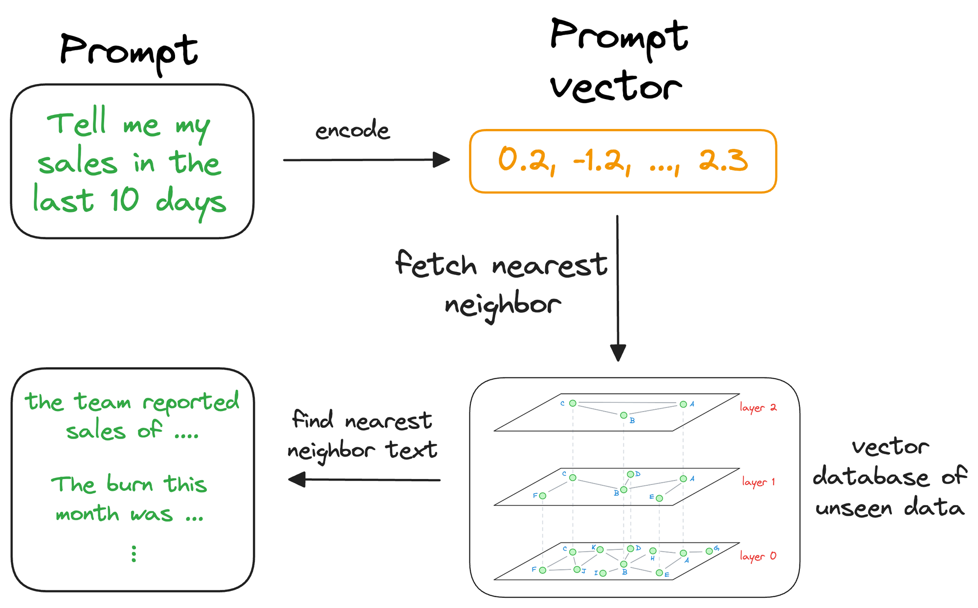
This search process retrieves context that is similar to the query vector, which represents the context or topic the LLM is interested in.

We can augment this retrieved content along with the actual prompt provided by the user and give it as input to the LLM.

Consequently, the LLM can easily incorporate this info while generating text because it now has the relevant details available in the prompt.

And...Congratulations!

You just learned Retrieval-Augmented Generation (RAG). I am sure you must have heard this term many times now and what we discussed above is the entire idea behind RAG.

I intentionally did not mention RAG anywhere earlier to build the desired flow and avoid intimidating you with this term first.

In fact, even its name entirely justifies what we do with this technique:

• Retrieval: Accessing and retrieving information from a knowledge source, such as a database or memory.
• Augmented: Enhancing or enriching something, in this case, the text generation process, with additional information or context.
• Generation: The process of creating or producing something, in this context, generating text or language.

Another critical advantage of RAG is that it drastically helps the LLM reduce hallucinations in its responses. I am sure you must have heard of this term too somewhere.

Hallucinations happen when a language model generates information that is not grounded in reality or when it makes up things.

This can lead to the model generating incorrect or misleading information, which can be problematic in many applications.

With RAG, the language model can use the retrieved information (which is expected to be reliable) from the vector database to ensure that its responses are grounded in real-world knowledge and context, reducing the likelihood of hallucinations.

This makes the model's responses more accurate, reliable, and contextually relevant, improving its overall performance and utility.

This idea makes intuitive sense as well.

Vector database providers

These days, there are tons of vector database providers, which can help us store and retrieve vector representations of our data efficiently.

• Pinecone: Pinecone is a managed vector database service that provides fast, scalable, and efficient storage and retrieval of vector data. It offers a range of features for building AI applications, such as similarity search and real-time analytics.
• Weaviate: Weaviate is an open-source vector database that is robust, scalable, cloud-native, and fast. With Weaviate, one can turn your text, images, and more into a searchable vector database using state-of-the-art ML models.
• Milvus: Milvus is an open-source vector database built to power embedding similarity search and AI applications. Milvus makes unstructured data search more accessible and provides a consistent user experience regardless of the deployment environment.
• Qdrant: Qdrant is a vector similarity search engine and vector database. It provides a production-ready service with a convenient API to store, search, and manage points—vectors with an additional payload. Qdrant is tailored to extended filtering support. It makes it useful for all sorts of neural network or semantic-based matching, faceted search, and other applications.

Pinecone demo

Going ahead, let’s get into some practical details on how we can index vectors in a vector database and perform search operations over them.

For this demonstration, I will be using Pinecone as it’s possibly one of the easiest to begin with and understand. But many other provides are linked above, which you can explore if you wish to.

To begin, we first install a few dependencies, like Pinecone and Sentence transformers:

It is important to encode this text dataset into vector embeddings to store them in the vector database. For this purpose, we will leverage the SentenceTransformers library.

It provides pre-trained transformer-based architectures that can efficiently encode text into dense vector representations, often called embeddings.

The SentenceTransformers model offers various pre-trained architectures, such as BERT, RoBERTa, and DistilBERT, fine-tuned specifically for sentence embeddings.

These embeddings capture semantic similarities and relationships between textual inputs, making them suitable for downstream tasks like classification and clustering.

DistilBERT is a relatively smaller model, so we shall be using it in this demonstration.

Next, open a Jupyter Notebook and import the above libraries:

Moving on, we download and instantiate the DistilBERT sentence transformer model as follows:

To get started with Pinecone and create a vector database, we need a Pinecone API key.

To get this, head over to the Pinecone website and create an account here: https://app.pinecone.io/?sessionType=signup. We get to the following page after signing up:

Grab your API key from the left panel in the dashboard below:

Click on API Keys -> Create API Key -> Enter API Key Name -> Create.

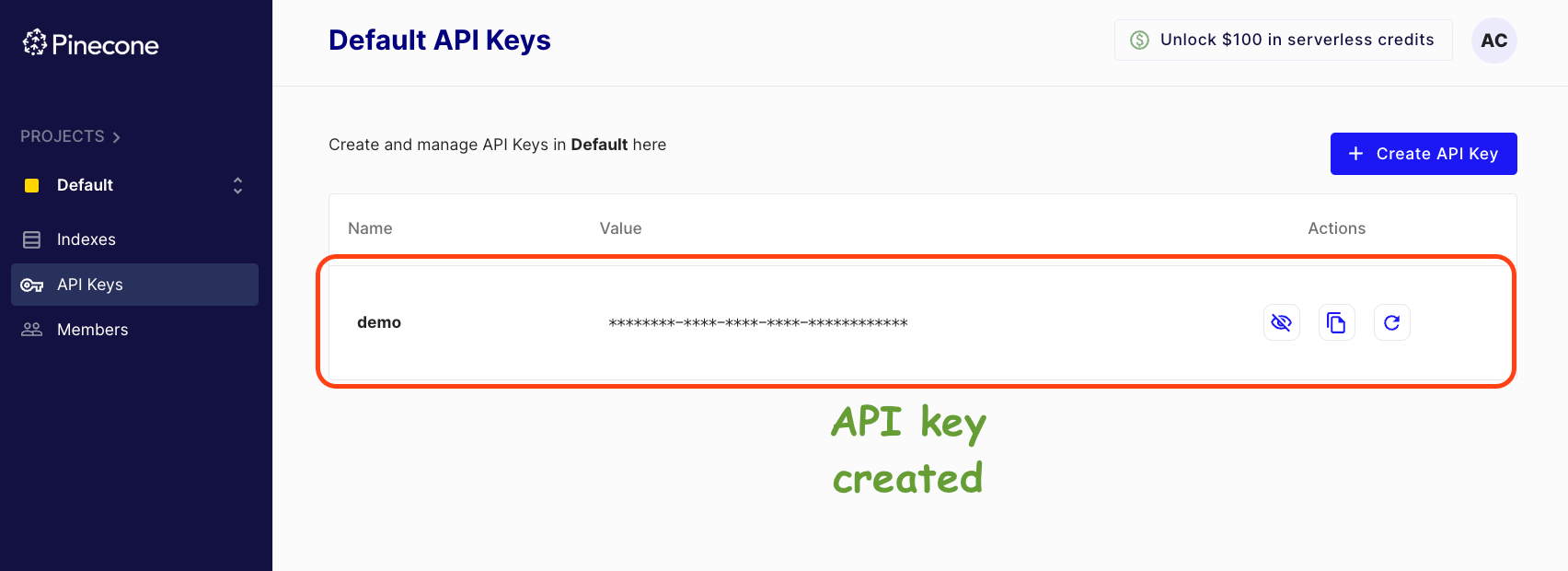
Done!

Grab this API key (like the copy to clipboard button), go back to the Jupyter Notebook, and establish a connection to Pinecone using this API Key, as follows:

In Pinecone, we store vector embeddings in indexes. The vectors in any index we create must share the same dimensionality and distance metric for measuring similarity.

We create an index using the create_index() method of the Pinecone class object created above.

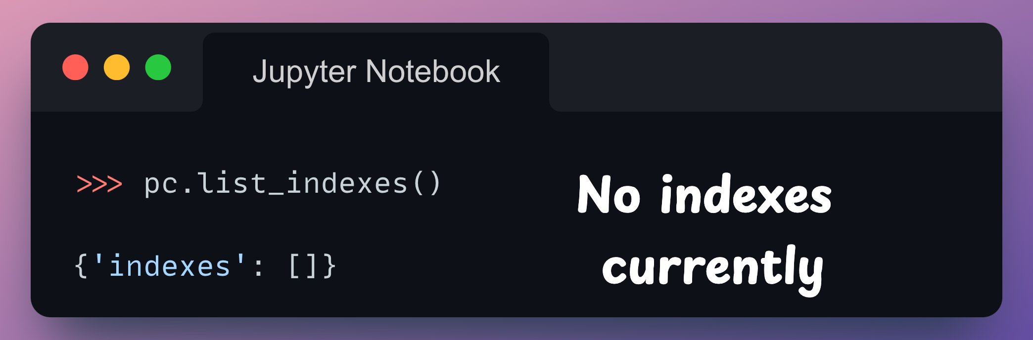
On a side note, currently, as we have no indexes, running the list_indexes() method returns an empty list in the indexes key of the dictionary:

Coming back to creating an index, we use the using the create_index() method of the Pinecone class object as follows:

Here’s a breakdown of this function call:

• name: The name of the index. This is a user-defined name that can be used to refer to the index later when performing operations on it.
• dimension: The dimensionality of the vectors that will be stored in the index. This should match the dimensionality of the vectors that will be inserted into the index. We have specified 768 here because that is the embedding dimension returned by the SentenceTransformer model.
• metric: The distance metric used to calculate the similarity between vectors. In this case, euclidean is used, which means that the Euclidean distance will be used as the similarity metric.
• spec: A PodSpec object that specifies the environment in which the index will be created. In this example, the index is created in a GCP (Google Cloud Platform) environment named gcp-starter.

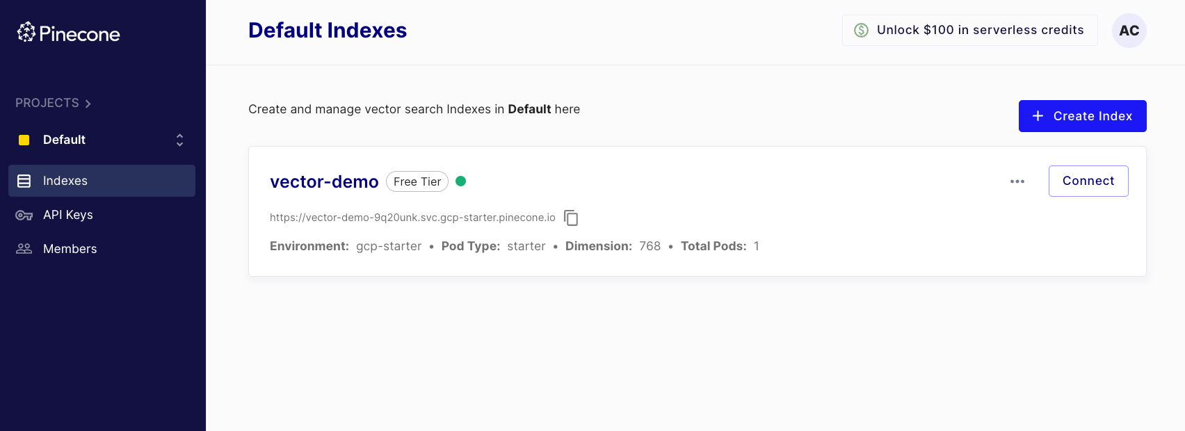
Executing this method creates an index, which we can also see in the dashboard:

Now that we have created an index, we can push vector embeddings.

To do this, let’s create some text data and encode it using the SentenceTransformer model.

I have created a dummy data below:

We create embeddings for these sentences as follows:

This code snippet iterates over each sentence in the data list we defined earlier and encodes the text of each sentence into a vector using the downloaded sentence transformer model (model).

It then creates a dictionary vector_info containing the sentence ID (id) and the corresponding vector (values), and appends this dictionary to the vector_data list.

In practical instances, there can be multiple indexes under the same account, we must create an index object that specifies the index we wish to add these embeddings to. This is done as follows:

Now that we have the embeddings and the index, we upsert these vectors.

Upsert is a database operation that combines the actions of update and insert. It inserts a new document into a collection if the document does not already exist, or updates an existing document if it does exist. Upsert is a common operation in databases, especially in NoSQL databases, where it is used to ensure that a document is either inserted or updated based on its existence in the collection.

Done!

We have added these vectors to the index. While the output does highlight this, we can double verify this by using the describe_index_stats operation to check if the current vector count matches the number of vectors we upserted:

Here's what each key in the returned dictionary represents:

• dimension: The dimensionality of the vectors stored in the index (768, in this case).
• index_fullness: A measure of how full the index is, typically indicating the percentage of slots in the index that are occupied.
• namespaces: A dictionary containing statistics for each namespace in the index. In this case, there is only one namespace ('') with a vector_count of 10, indicating that there are 10 vectors in the index.
• total_vector_count: The total number of vectors in the index across all namespaces (10, in this case).

Now that we have stored the vectors in the above index, let’s run a similarity search to see the obtained results.

We can do this using the query() method of the index object we created earlier.

First, we define a search text and generate its embedding:

Next, we query this as follows:

This code snippet calls the query method on an index object, which performs a nearest neighbor search for a given query vector (search_embedding) and returns the top 3 matches.

Here's what each key in the returned dictionary represents:

• matches: A list of dictionaries, where each dictionary contains information about a matching vector. Each dictionary includes the id of the matching vector, the score indicating the similarity between the query vector and the matching vector. As we specified euclidean as our metric while creating this index, a higher score indicates more distance or similarity.
• namespace: The namespace of the index where the query was performed. In this case, the namespace is an empty string (''), indicating the default namespace.
• usage: A dictionary containing information about the usage of resources during the query operation. In this case, read_units indicates the number of read units consumed by the query operation, which is 5. However, we originally appended 10 vectors to this index, which shows that it did look through all the vectors to find the nearest neighbors.

From the above results, we notice that the top 3 neighbors of the search_text ("Vector database are really helpful") are:

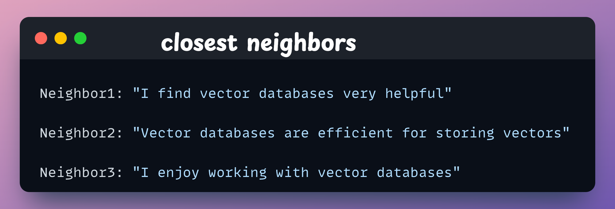
Awesome!

Conclusion

With this, we come to an end to this deep dive into vector databases.

To recap, we learned that vector databases are specialized databases designed to efficiently store and retrieve vector representations of data.

By organizing vectors into indexes, vector databases enable fast and accurate similarity searches, making them invaluable for tasks like recommendation systems and information retrieval.

Moreover, the Pinecone demo showcased how easy it is to create and query a vector index using Pinecone's service.

Before I end this article, there’s one important point I want to mention.

Just because vector databases sound cool, it does not mean that you have to adopt them in each and every place where you wish to find vector similarities.

It's so important to assess whether using a vector database is necessary for your specific use case.

For small-scale applications with a limited number of vectors, simpler solutions like NumPy arrays and doing an exhaustive search will suffice.

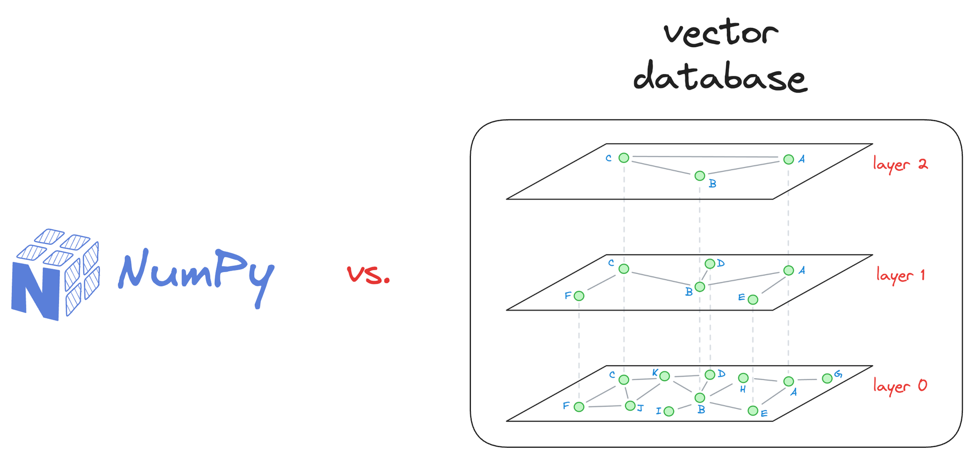
There’s no need to move to vector databases unless you see any benefits, such as latency improvement in your application, cost reduction, and more.

I hope you learned something new today!

I know we discussed many details in this deep dive, so if there’s any confusion, feel free to post them in the comments.

Or, if you wish to connect privately, feel free to initiate a chat here:

Thanks for reading!

If you loved reading this deep dive, I am sure you will learn a lot of practical skills from other rich deep dives too, like these:

Federated Learning: A Critical Step Towards Privacy-Preserving Machine Learning

Learn real-world ML model development with a primary focus on data privacy – A practical guide.

Daily Dose of Data ScienceAvi Chawla

You Cannot Build Large Data Projects Until You Learn Data Version Control!

The underappreciated, yet critical, skill that most data scientists overlook.

Daily Dose of Data ScienceAvi Chawla

Why Bagging is So Ridiculously Effective At Variance Reduction?

Diving into the mathematical motivation for using bagging.

Daily Dose of Data ScienceAvi Chawla

Become a full member (if you aren't already) so that you never miss an article: