ARQ: A New Structured Reasoning Approach for LLMs

LLMs

ARQ: A New Structured Reasoning Approach for LLMs

Researchers have open-sourced a new reasoning approach that actually prevents hallucinations in LLMs.

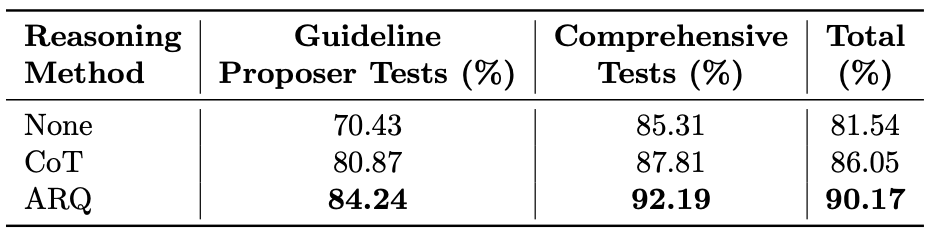
It beats popular techniques like Chain-of-Thought and has a SOTA success rate of 90.2%.

It’s implemented in the Parlant open-source framework to build instruction-following Agents (GitHub repo).

Here’s the core problem with current techniques that this new approach solves.

We have enough research to conclude that LLMs often struggle to assess what truly matters in a particular stage of a long, multi-turn conversation.

For instance, when you give Agents a 2,000-word system prompt filled with policies, tone rules, and behavioral dos and don’ts, you expect them to follow it word by word.

But here’s what actually happens:

• They start strong initially.
• Soon, they drift and start hallucinating.
• Shortly after, they forget what was said five turns ago.
• And finally, the LLM that was supposed to “never promise a refund” is happily offering one.

This means they can easily ignore crucial rules (stated initially) halfway through the process.

We expect techniques like Chain-of-Thought will help.

But even with methods like CoT, reasoning remains free-form, i.e., the model “thinks aloud” but it has limited domain-specific control.

That’s the exact problem the new technique, called Attentive Reasoning Queries (ARQs), solves.

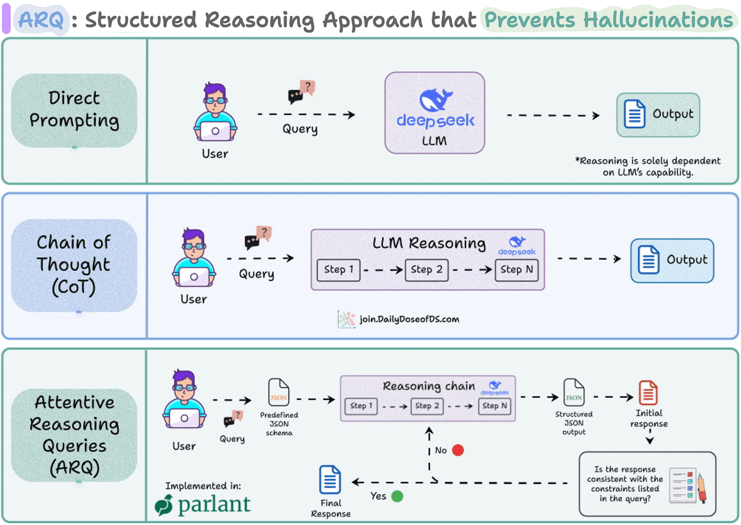
Instead of letting LLMs reason freely, ARQs guide them through explicit, domain-specific questions.

Essentially, each reasoning step is encoded as a targeted query inside a JSON schema.

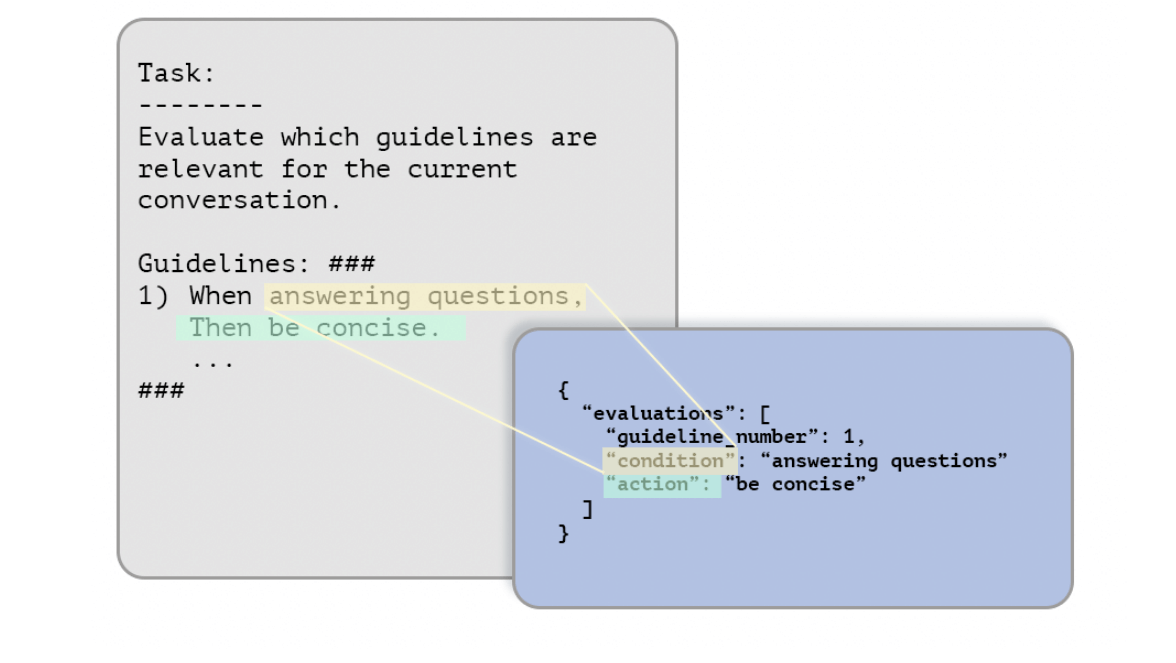
For example, before making a recommendation or deciding on a tool call, the LLM is prompted to fill structured keys like:

{
  “current_context”: “Customer asking about refund eligibility”,
  “active_guideline”: “Always verify order before issuing refund”,
  “action_taken_before”: false,
  “requires_tool”: true,
  “next_step”: “Run check_order_status()”
}

This type of query does two things:

1. Reinstate critical instructions by keeping the LLM aligned mid-conversation.
2. Facilitate intermediate reasoning, so that the decisions are auditable and verifiable.

By the time the LLM generates the final response, it’s already walked through a sequence of *controlled* reasoning steps, which did not involve any free text exploration (unlike techniques like CoT or ToT).

Here’s the success rate across 87 test scenarios:

• ARQ → 90.2%
• CoT reasoning → 86.1%
• Direct response generation → 81.5%

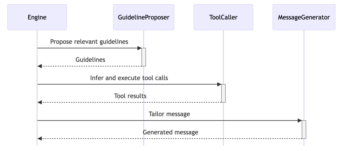
This approach is actually implemented in Parlant, a recently trending open-source framework to build instruction-following Agents (14k stars).

ARQs are integrated into three key modules:

• Guideline proposer to decide which behavioral rules apply.
• Tool caller to determine what external functions to use.
• Message generator, when it produces the final customer-facing reply.

You can see the full implementation and try it yourself.

But the core insight applies regardless of what tools you use:

When you make reasoning explicit, measurable, and domain-aware, LLMs stop improvising and start reasoning with intention. Free-form thinking sounds powerful, but in high-stakes or multi-turn scenarios, structure always wins.

You can find the Parlant GitHub repo here →

machine learning

​The intuition behind using ‘Variance’ in PCA​​

PCA is built on the idea of variance preservation.

The more variance we retain when reducing dimensions, the less information is lost.

Here’s an intuitive explanation of this.

Imagine you have the following data about three people:

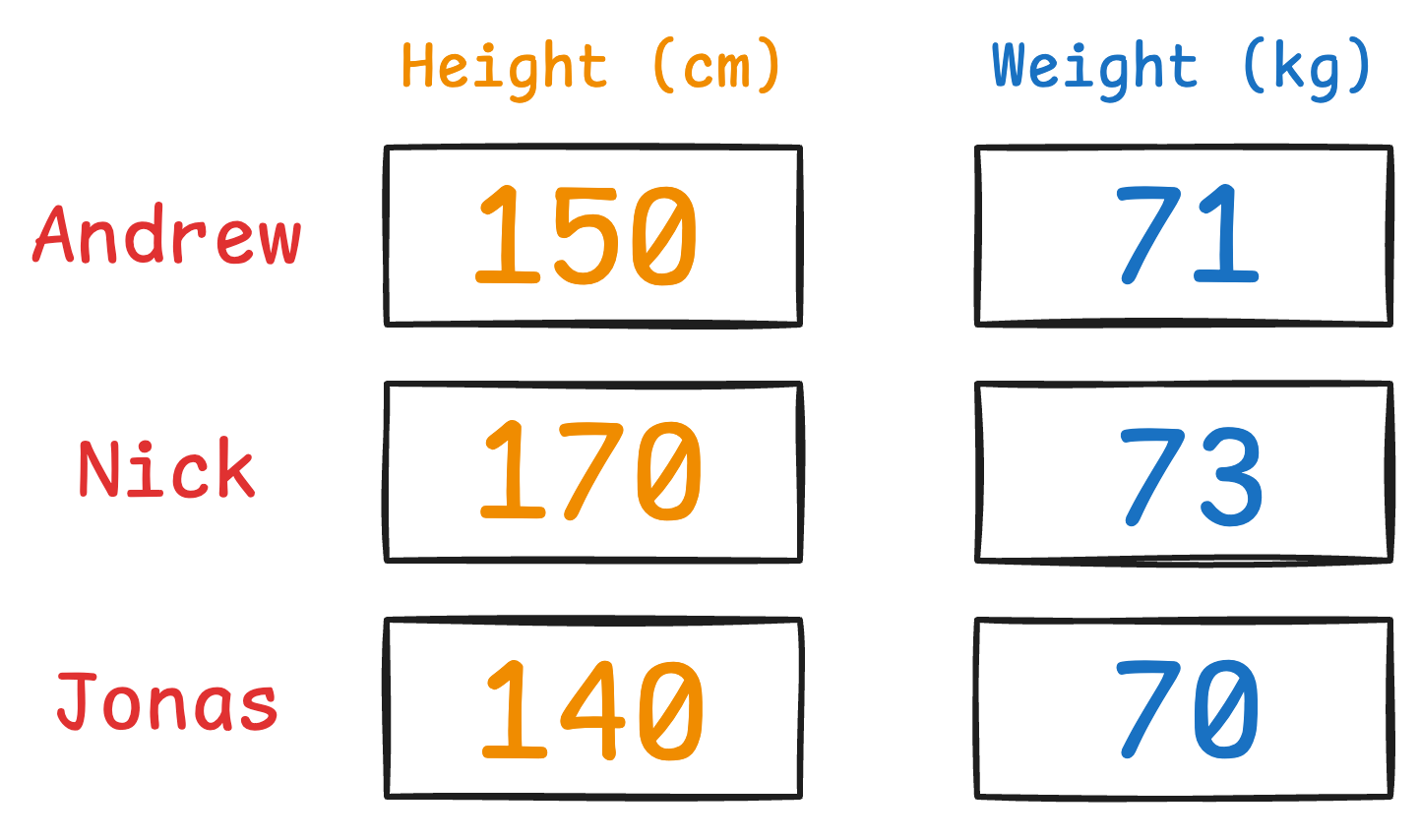
It is clear that height has more variance than weight.

Even if we discard the weight, we can still identify them solely based on height.

But if we discard the height, it’s a bit difficult to identify them now:

This is the premise on which PCA is built.

More specifically, during dimensionality reduction, if we retain more original data variance, we retain more information.

Of course, since it uses variance, it is influenced by outliers.

That said, in PCA, we don’t just measure column-wise variance and drop the columns with the least variance.

Instead, we transform the data to create uncorrelated features and then drop the new features based on their variance.

To dive into more mathematical details, we formulated the entire PCA algorithm from scratch here: ​Formulating PCA Algorithm From Scratch​, where we covered:

• What are vector projections, and how do they alter the mean and variance of the data?
• What is the optimization step of PCA?
• What are Lagrange Multipliers?
• How are Lagrange Multipliers used in PCA optimization?
• What is the final solution obtained by PCA?
• Proving that the new features are indeed uncorrelated.
• How to determine the number of components in PCA?
• What are the advantages and disadvantages of PCA?
• Key takeaways.

And in the follow-up part to PCA, we formulated tSNE from scratch, an algorithm specifically designed to visualize high-dimensional datasets.

We also implemented tSNE with all its backpropagation steps from scratch using NumPy.

Read here: ​Formulating and Implementing the t-SNE Algorithm From Scratch.​​

machine learning

​A point of caution when using one-hot encoding​

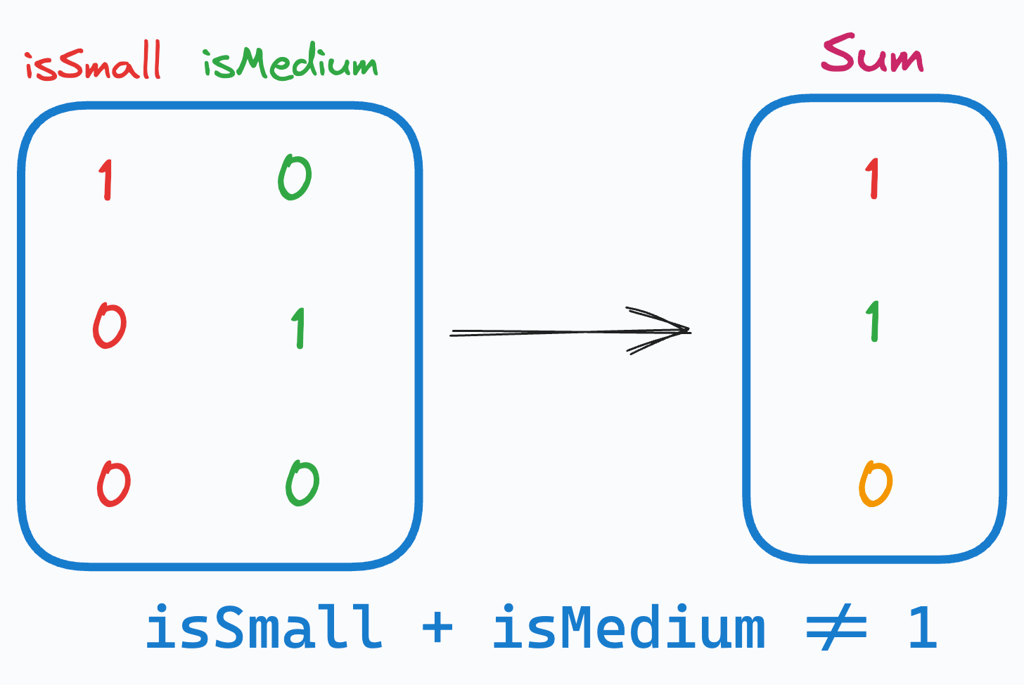
One-hot encoding introduces a problem in the dataset.

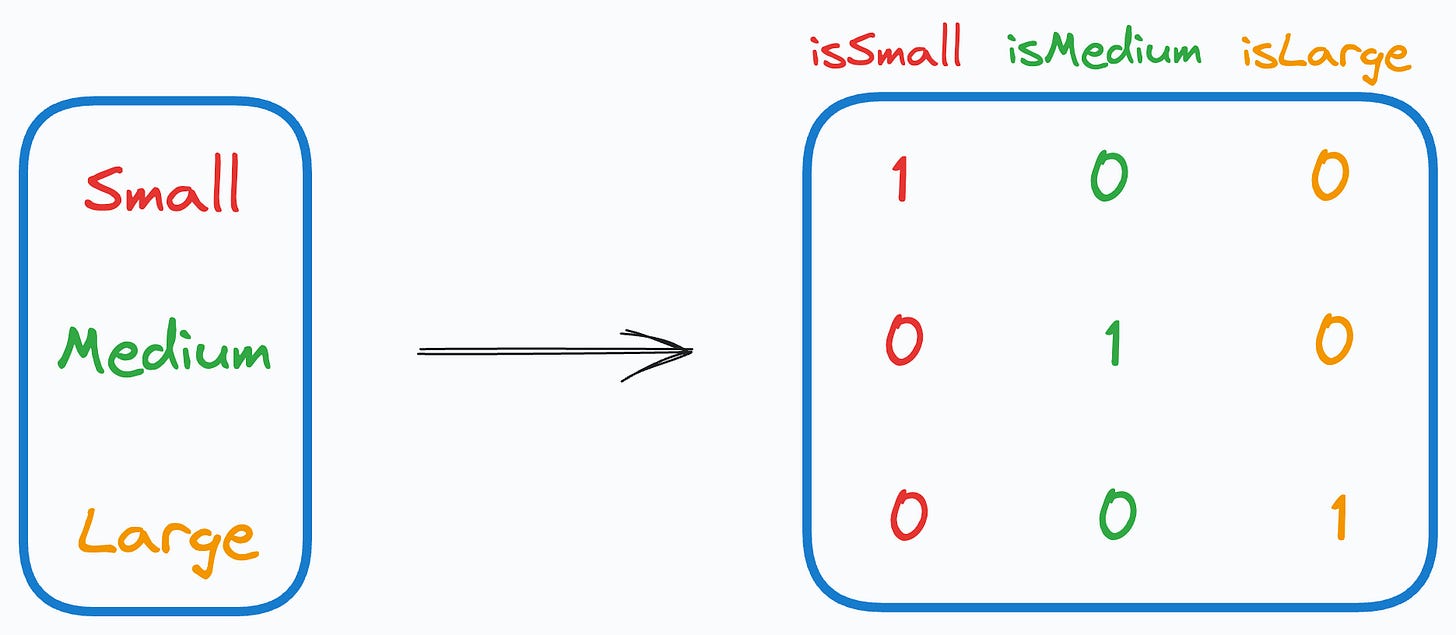
More specifically, when we use it, we unknowingly introduce perfect multicollinearity.

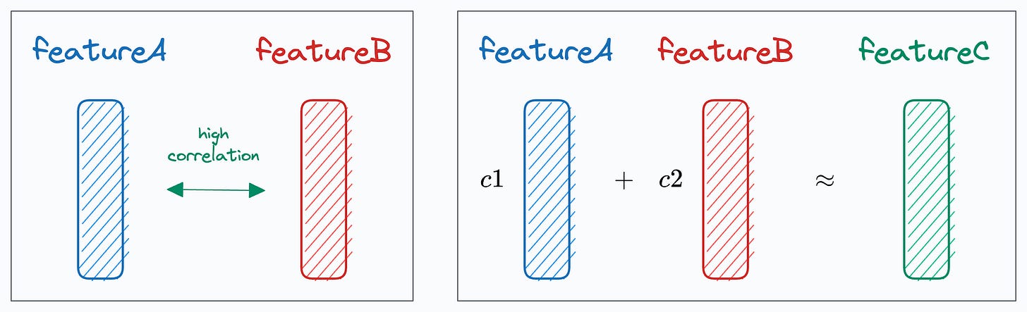
Multicollinearity arises when two (or more) features are highly correlated OR two (or more) features can predict another feature:

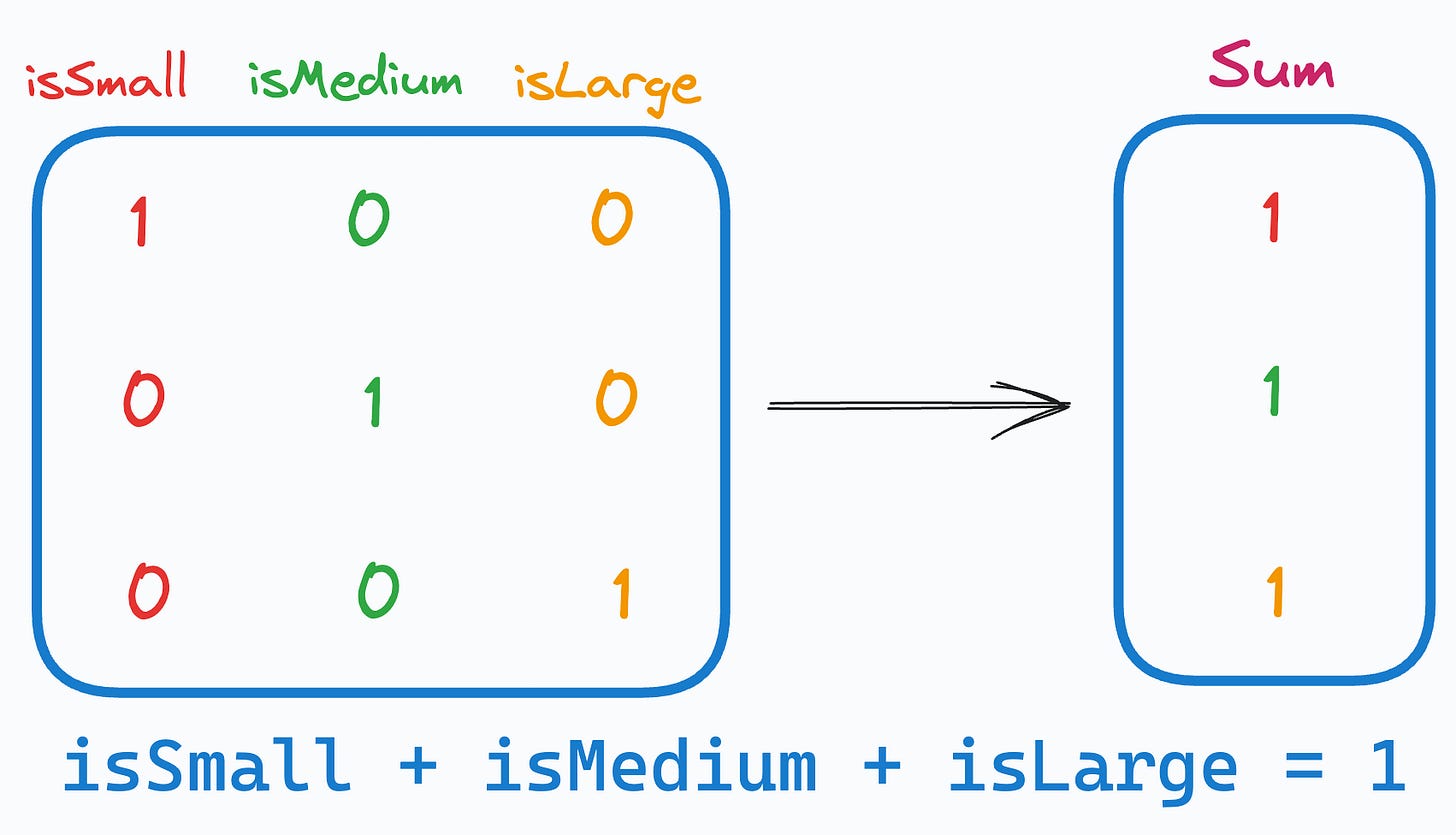
In our case, as the sum of one-hot encoded features is always 1, it leads to perfect multicollinearity, and it can be problematic for models that don’t perform well under such conditions.

This problem is often called the Dummy Variable Trap.

Talking specifically about linear regression, for instance, it is bad because:

• In some way, our data has a redundant feature.
• Regression coefficients aren’t reliable in the presence of multicollinearity, etc.

That said, the solution is pretty simple.

Drop any arbitrary feature from the one-hot encoded features.

This instantly mitigates multicollinearity and breaks the linear relationship that existed before, as depicted below:

The above way of categorical data encoding is also known as dummy encoding, and it helps us eliminate the perfect multicollinearity introduced by one-hot encoding.

​We covered 8 fatal (yet non-obvious) pitfalls (with measures) in DS here →