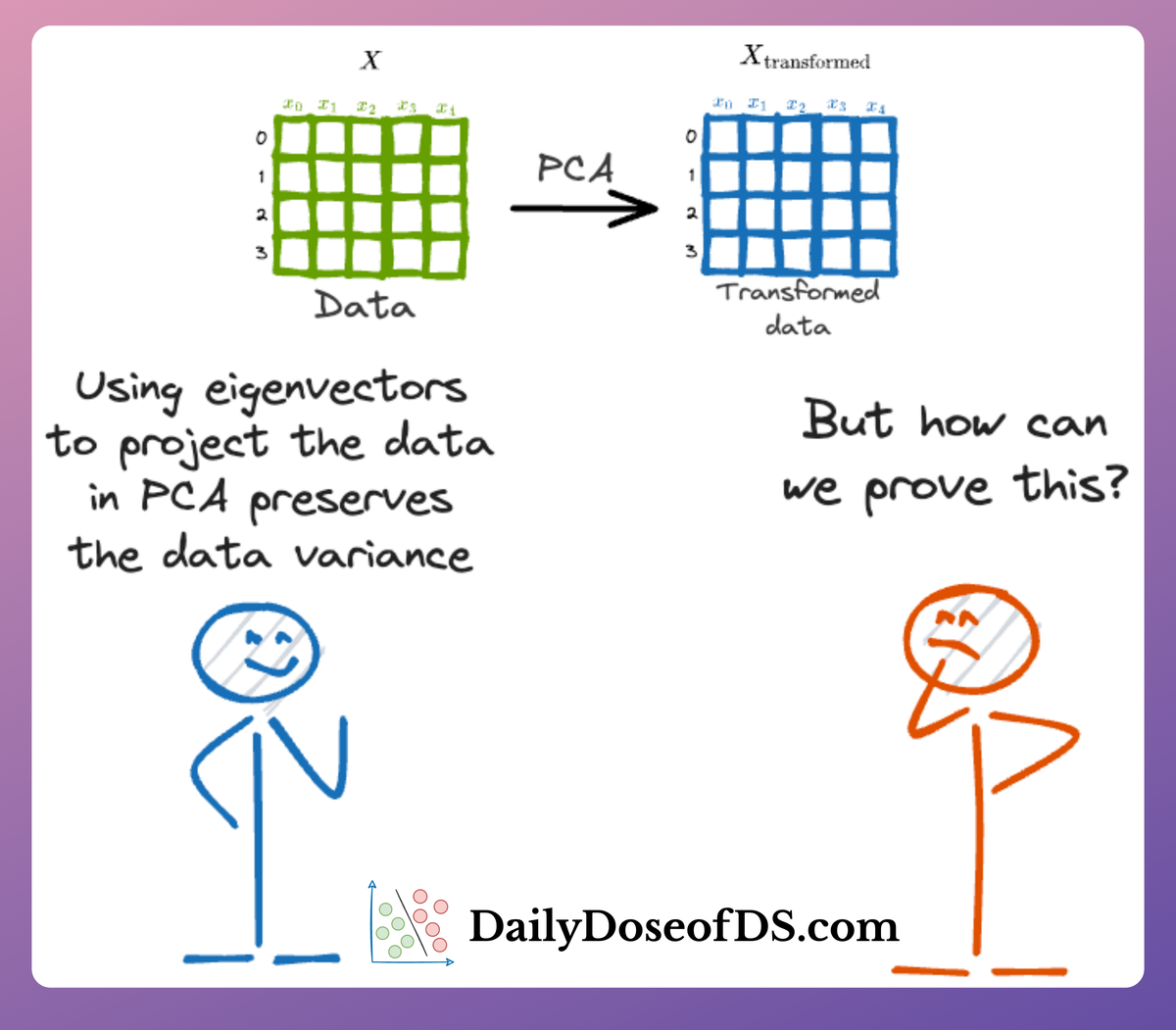
PCA
Sparse Random Projections
An alternative to PCA for highly dimensional datasets.

Avi Chawla
An alternative to PCA for highly dimensional datasets.

TODAY'S ISSUE
This is the time complexity of PCA:
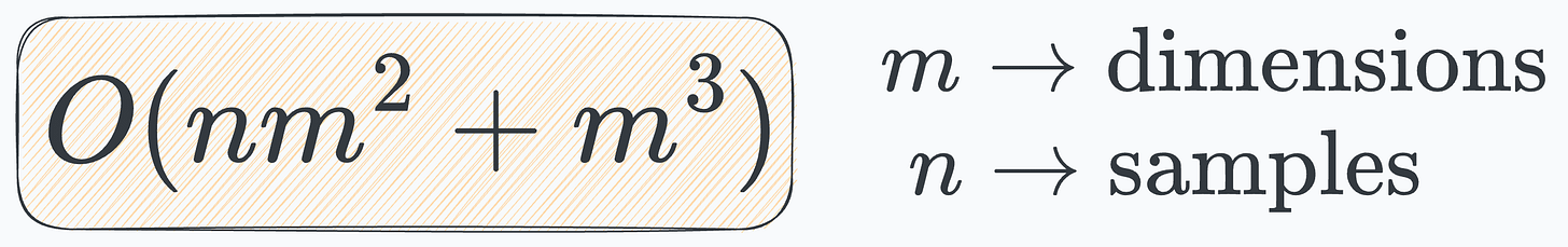
The cubic relationship with the number of dimensions makes it impractical on high-dimensional datasets, say, 1000d, 2000d, and more.
I find it quite amusing about PCA.
Think about it: You want to reduce the dimension, but the technique itself isn’t feasible when you have lots of dimensions.
Anyway…
Sparse random projection is a pretty fine solution to handle this problem.
Let me walk you through the intuition before formally defining it.
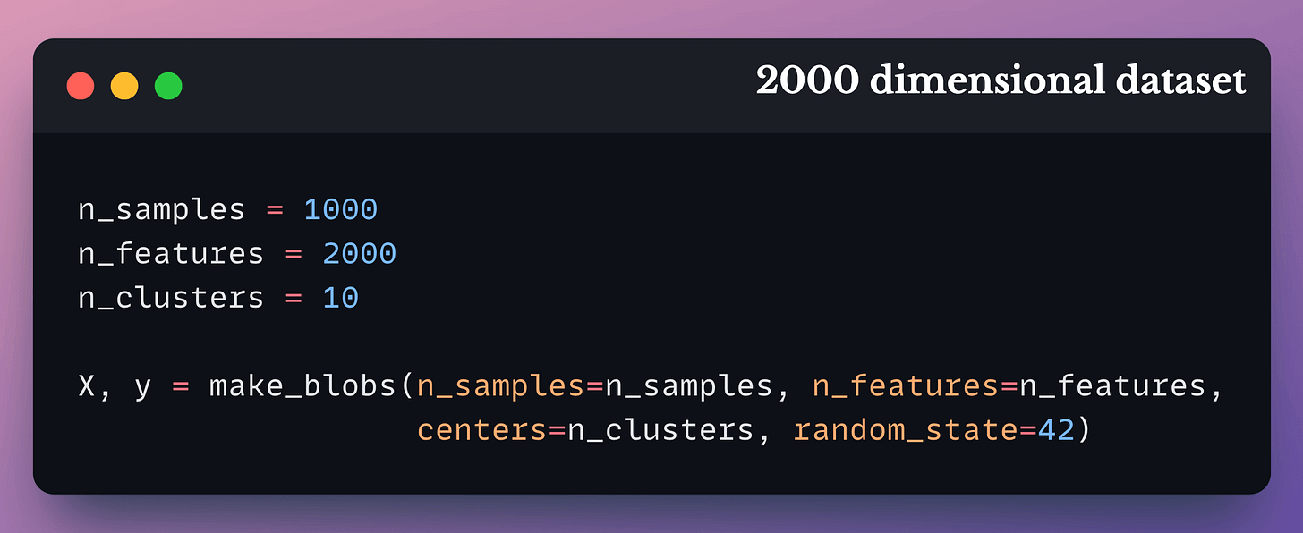
Consider the following 2000-dimensional dataset:
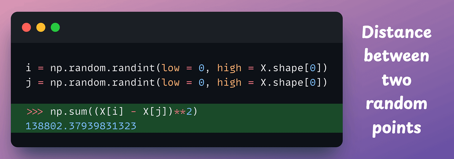
Let’s find the distance between two random points here:
Now imagine multiplying the above high-dimensional matrix X with a random projection matrix M of shape (m, d), which results in the projected matrix:
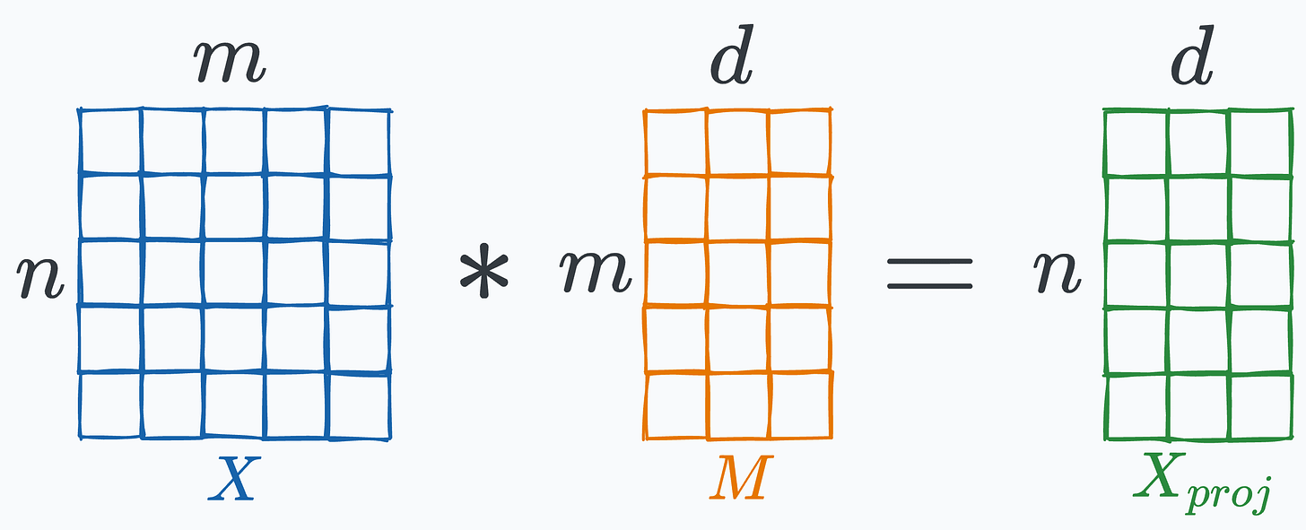
In this case, I projected X to 1000 dimensions from 2000 dimensions.
Now, if we find the distance between the same two points again, we get this:
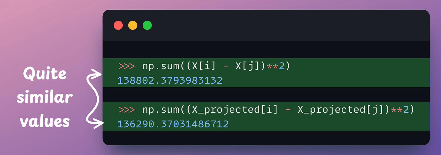
The two distance values are quite similar, aren’t they?
This hints that if we have a pretty high-dimensional dataset, we can transform it to a lower dimension while almost preserving the distance between any two points.
If you read the deep dive on the curse of dimensionality, we covered the mathematical details behind why distance remains almost preserved.
But let’s not stop there since we also need to check if the projected data is any useful.
Recall that we created a blobs dataset.
So let’s utilize KMeans on both the high-dimensional original data and the projected data, and measure the clustering quality using silhouette score.
X is implemented below: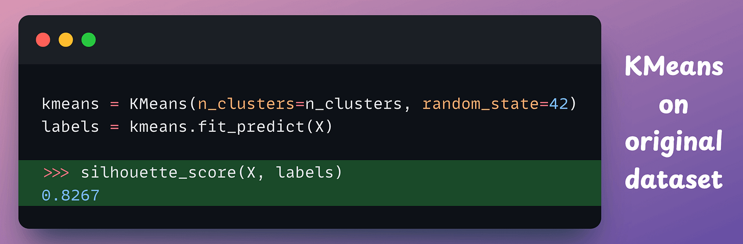
X_projected is implemented below (for random projection, we make use of SparseRandomProjection from sklearn):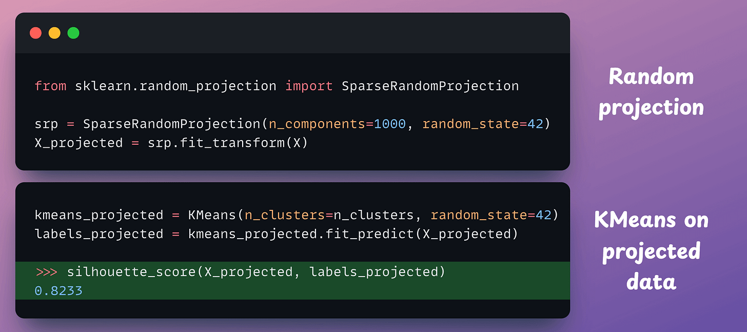
Look at the silhouette scores:
X, we get 0.8267 (the higher, the better).These two scores are highly similar, which indicates that both datasets produce a similar quality of clustering.
Formally speaking, random projections allow us to project high-dimensional datasets into relatively lower-dimensional spaces while almost preserving the distance between the data points.
This has a mathematical intuition attached to it as well, which we covered here: A mathematical deep dive on the curse of dimensionality.
I mentioned “relatively” above since this won’t work if the two spaces significantly differ in their dimensionality.
I ran the above experiment on several dimensions, and the results are shown below:
Original:
Silhouette = 0.8267

Projected:
Components = 2000, Silhouette = 0.8244
Components = 1500, Silhouette = 0.8221
Components = 1000, Silhouette = 0.8233
Components = 750,  Silhouette = 0.8232
Components = 500,  Silhouette = 0.8158
Components = 300,  Silhouette = 0.8212
Components = 200,  Silhouette = 0.8207
Components = 100,  Silhouette = 0.8102
Components = 50,   Silhouette = 0.8041
Components = 20,   Silhouette = 0.7783
Components = 10,   Silhouette = 0.6491
Components = 5,    Silhouette = 0.6665
Components = 2,    Silhouette = 0.5108
From the above results, it is clear that as the dimension we project the data to decreases, the clustering quality drops, which makes intuitive sense as well.
Thus, the dimension you should project to becomes a hyperparameter you can tune based on your specific use case and dataset.
In my experience, random projections produce highly unstable results when the data you begin with is low-dimensional (<100 dimensions).
Thus, I only recommend it when the number of features is huge, say 700-800+, and PCA’s run-time is causing problems.
That said, random projection is also used in an LLM fine-tuning technique called VeRA:
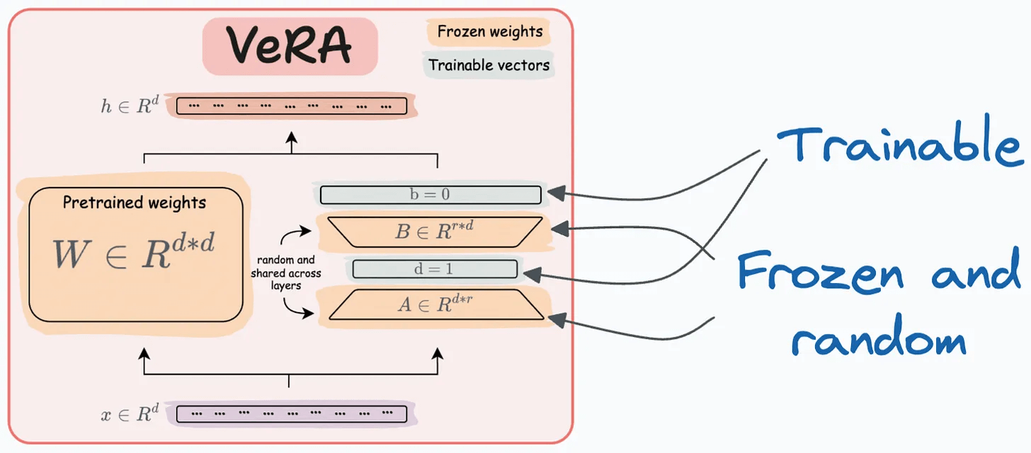
Recall that in LoRA, every layer has a different pair of low-rank matrices A and B, and both matrices are trained.
In VeRA, however, matrices A and B are frozen, random, and shared across all model layers. VeRA focuses on learning small, layer-specific scaling vectors, denoted as b and d, which are the only trainable parameters in this setup.
We covered 5 LLM fine-tuning techniques here:
Also, we formulated PCA from scratch (with all underlying mathematical details) here:
👉 Over to you: What are some ways to handle high-dimensional datasets when you want to use PCA?
One critical problem with the traditional RAG system is that questions are not semantically similar to their answers.
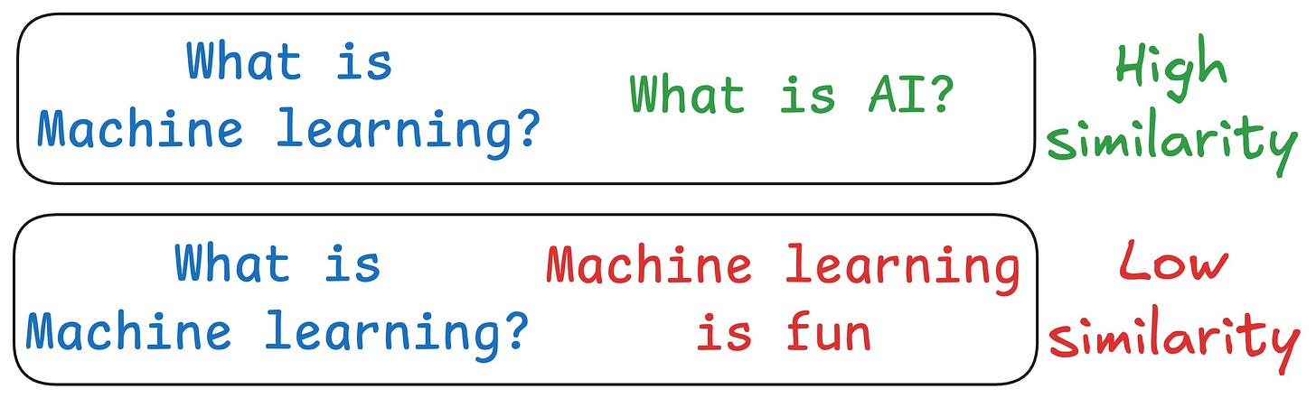
As a result, several irrelevant contexts get retrieved during the retrieval step due to a higher cosine similarity than the documents actually containing the answer.
HyDE solves this.
The following visual depicts how it differs from traditional RAG and HyDE.
We covered this in detail in a newsletter issue published last week →
If you have used DeepSeek-R1 (or any other reasoning model), you must have seen that they autonomously allocate thinking time before producing a response.
Last week, we shared how to embed reasoning capabilities into any LLM.
We trained our own reasoning model like DeepSeek-R1 (with code).
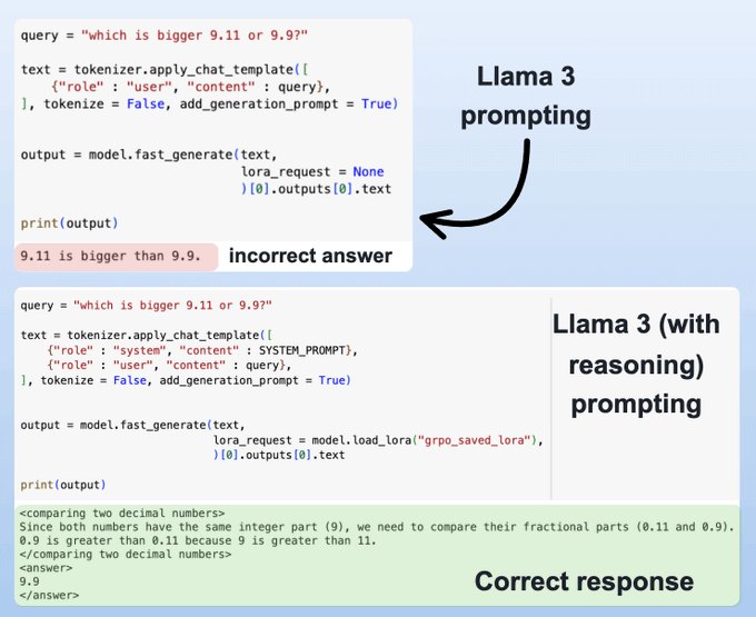
To do this, we used:
Find the implementation and detailed walkthrough newsletter here →