Machine Learning
KernelPCA vs. PCA
...and when to not use KernelPCA

Avi Chawla
...and when to not use KernelPCA

TODAY'S ISSUE
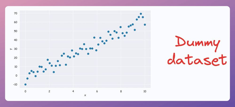
During dimensionality reduction, principal component analysis (PCA) tries to find a low-dimensional linear subspace that the given data conforms to.
For instance, consider the following dummy dataset:
It’s pretty clear from the above visual that there is a linear subspace along which the data could be represented while retaining maximum data variance. This is shown below:
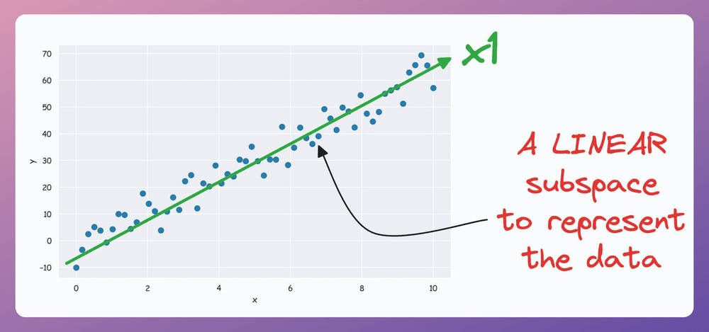
But what if our data conforms to a low-dimensional yet non-linear subspace?
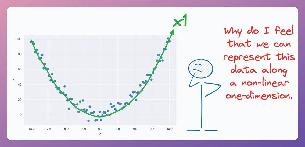
For instance, consider the following dataset:
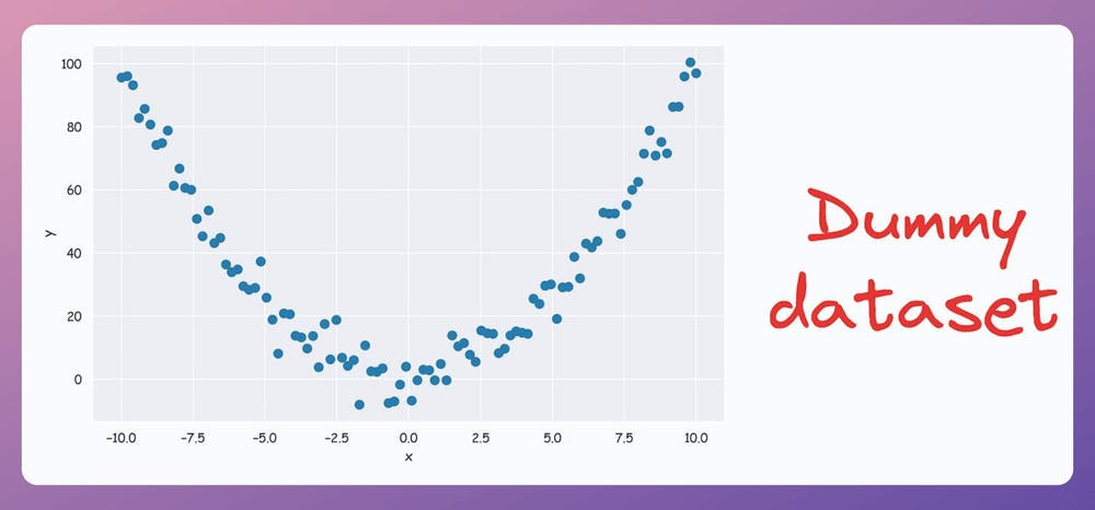
Do you see a low-dimensional non-linear subspace along which our data could be represented?
No?
Don’t worry. Let me show you!
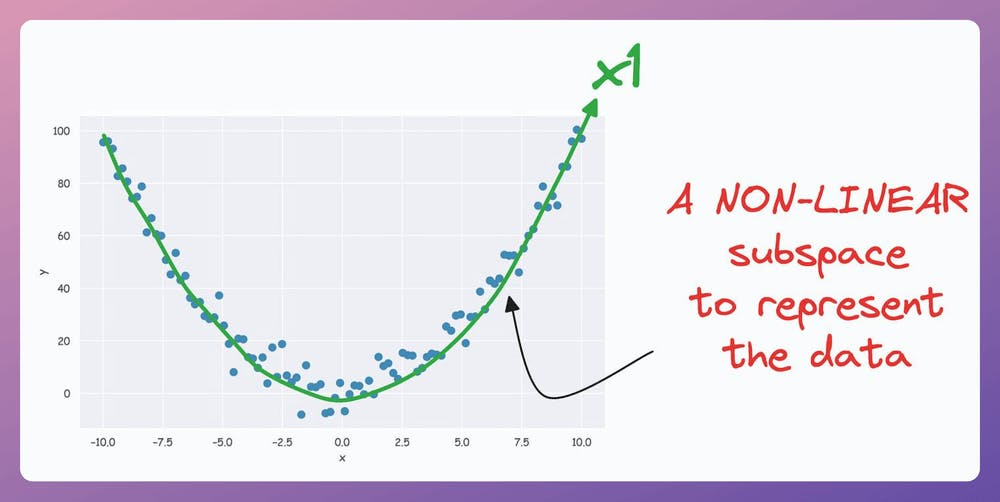
The above curve is a continuous non-linear and low-dimensional subspace that we could represent our data given along.
Okay…so why don’t we do it then?
The problem is that PCA cannot determine this subspace because the data points are non-aligned along a straight line.
In other words, PCA is a linear dimensionality reduction technique.
Thus, it falls short in such situations.
Nonetheless, if we consider the above non-linear data, don’t you think there’s still some intuition telling us that this dataset can be reduced to one dimension if we can capture this non-linear curve?
KernelPCA precisely addresses this limitation of PCA
The idea is pretty simple.
In standard PCA, we compute the eigenvectors and eigenvalues of the standard covariance matrix (we covered the mathematics here).
In KernelPCA, however:
p” components.If there's any confusion in the above steps, I would highly recommend reading this deep dive on PCA, where we formulated the entire PCA algorithm from scratch. It will help you understand the underlying mathematics.
That said, the efficacy of KernelPCA over PCA is evident from the demo below.
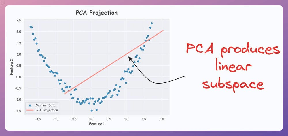
As shown below, even though the data is non-linear, PCA still produces a linear subspace for projection:
However, KernelPCA produces a non-linear subspace:
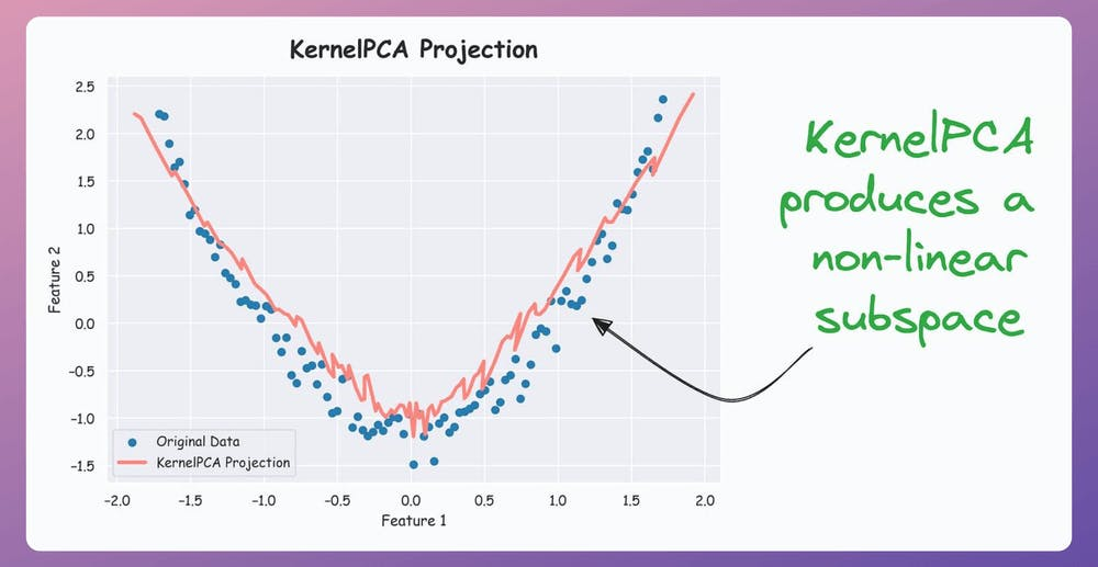
That's handy, isn't it?
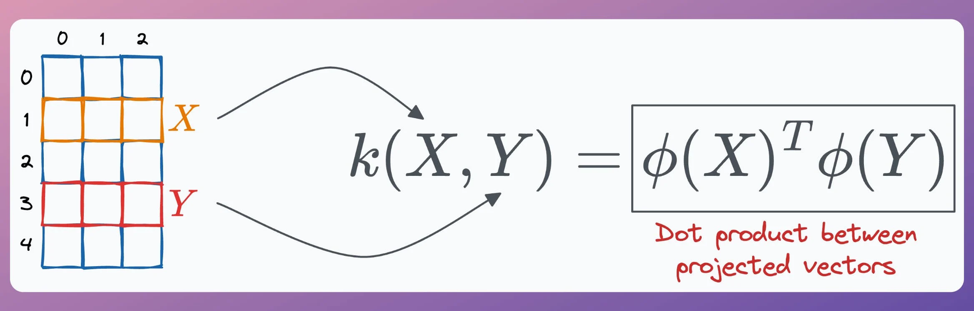
The catch here is the run time.
Since we compute the pairwise dot products in KernelPCA, this adds an additional O(n^2) time-complexity.
Thus, it increases the overall run time. This is something to be aware of when using KernelPCA.
If you want to dive into the clever mathematics of the kernel trick and why it is called a “trick,” we covered this in the newsletter here:
👉 Over to you: What are some other limitations of PCA?
There are many issues with Grid search and random search.
Bayesian optimization solves this.
It’s fast, informed, and performant, as depicted below:

Learning about optimized hyperparameter tuning and utilizing it will be extremely helpful to you if you wish to build large ML models quickly.
Linear regression makes some strict assumptions about the type of data it can model, as depicted below.

Can you be sure that these assumptions will never break?
Nothing stops real-world datasets from violating these assumptions.
That is why being aware of linear regression’s extensions is immensely important.
Generalized linear models (GLMs) precisely do that.
They relax the assumptions of linear regression to make linear models more adaptable to real-world datasets.