Evaluation: Fundamentals
LLMOps Part 9: A foundational guide to the evaluation of LLM applications, covering challenges and a practical taxonomy of evaluation methods.
Recap
In the previous chapter (LLMOps Part 8), we examined memory context and temporal awareness as critical components of context engineering within LLM systems.
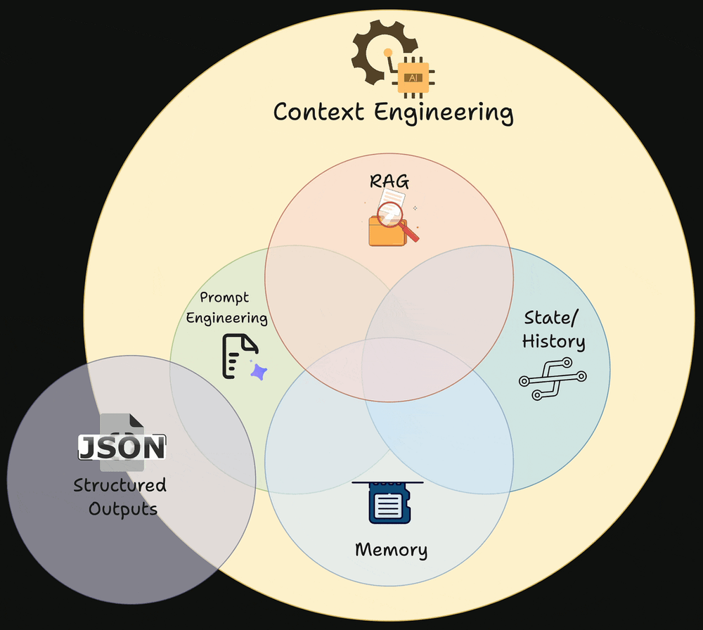
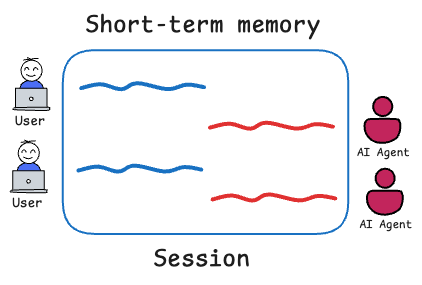
We began by drawing a clear distinction between short-term and long-term memory.
Short-term memory was defined as immediate context within the session or more precisely, what's part of the "active" prompt. It is ephemeral, bounded, and directly readable by the model. We discussed practical strategies such as last-N turns and rolling summaries pattern that preserves coherence while keeping token growth under control.
We then defined long-term memory as information retained across sessions or that persists even as short-term context moves on. It is implemented through external storage such as vector databases.
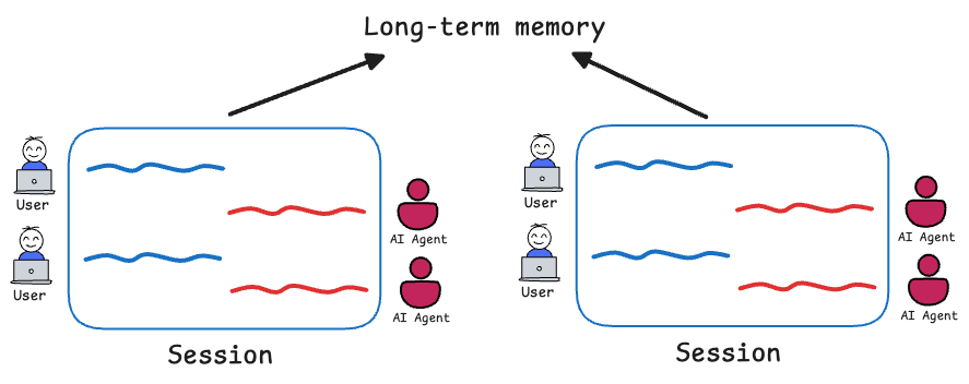
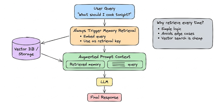
Here, we emphasized a critical architectural principle: persistent information is not automatically usable. It must be retrieved, filtered, and injected into working context before the model can reason over it. We also explored storage strategies, retrieval frequency, caching, pruning and cost considerations.
From there, we shifted to dynamic and temporal context injection. Unlike stored memory, dynamic context is not pre-authored or stored, but assembled or updated in real-time based on the current state.
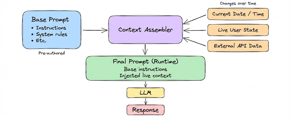
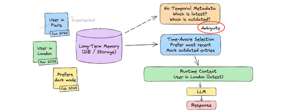
We showed how these injections move systems beyond static Q&A into adaptive, state-aware behavior. Here, temporal grounding for memory emerged as a central theme: without timestamps and recency-aware ranking, memory becomes unreliable. Time metadata transforms memory from an archive into a living representation of evolving user state.
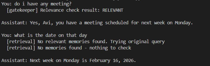
Next, we implemented a basic hands-on memory-enabled assistant. The system combined short-term memory (turns + summary), long-term semantic memory (ChromaDB + embeddings) with timestamps, dynamic time injection, query rewriting for retrieval, memory relevance gating, and audit logging. The goal was to expose the mechanics of storing, retrieving, summarizing, injecting, and governing memory in a transparent and inspectable way. By walking through each component, we built intuition about how memory systems behave under the hood.
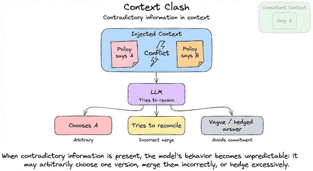
Finally, we addressed context failure modes that frequently arise when context is poorly engineered: context poisoning, distraction, clash, token wastage, and latency issues.
Altogether, the chapter reframed memory and dynamic context as engineered subsystems within LLM applications. Together, they extend the effective intelligence of the model and transform a stateless predictor into a stateful, adaptive and aware system.
If you haven’t yet gone through Part 8, we strongly recommend reviewing it first, as it helps maintain the natural learning flow of the series.
Read it here:
In this and the next few chapters, we will be exploring evaluation methods and approaches for LLM-based applications. This chapter, in particular, focuses on building a strong understanding of the fundamental concepts.
As always, every notion will be explained through clear examples and walkthroughs to develop a solid understanding.
Let’s begin!
Unique challenges in LLM evaluation
Evaluating LLMs is fundamentally different, and often harder, than evaluating traditional software or even classical ML models. Unlike a deterministic function or classifier, an LLM generates open-ended, probabilistic outputs in natural language.
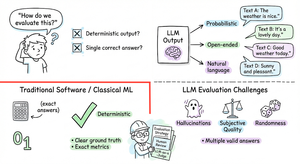
This introduces several challenges:
- Subjective and non-deterministic outputs: Many LLM tasks (creative writing, dialogue, etc.) don’t have a single objectively “correct” answer. An LLM’s response quality often lies on a spectrum, making strict pass/fail judgments difficult. Two answers can both be valid, or one may be “better” in style or clarity, a subjective call that’s hard to reduce to a simple metric. Moreover, identical prompts can yield different outputs on different runs due to randomness, so evaluation must account for variability.

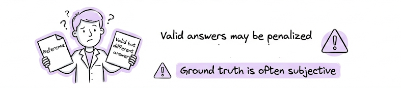
- Lack of ground truth: For tasks like open-ended Q&A, or chatbot behavior, we often lack a perfect ground truth. Often human references are also just one of many possible good outputs. This complicates reference-based evaluation, measuring model output just against a fixed reference might undervalue valid answers that differ in wording or approach.
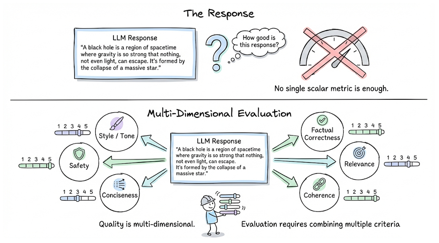
- Multifaceted quality criteria: The quality of an LLM output is multi-dimensional. It may need to be factually correct, relevant, coherent, concise, safe, stylistically appropriate, etc. No single scalar metric captures all these aspects. Hence evaluating “How good is this response?” often requires combining multiple criteria.
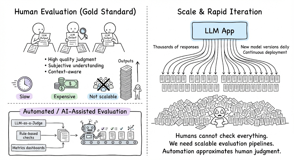
- Scale and automation needs: Human evaluation (e.g. having people read and score outputs) is considered the gold standard for subjective tasks, but it is slow, expensive, and not scalable for the rapid iteration cycles. LLM-driven applications might produce thousands of responses, or have new model versions daily. We can’t feasibly have humans check everything. We need automated or AI-assisted evaluation methods that approximate human judgment.
- Emergent behaviors and failure modes: LLMs can fail in unexpected ways, for example, hallucinating plausible-sounding but false information, making biased or toxic remarks, leaking system prompts, or failing on adversarial inputs. Evaluating these requires creative testing beyond standard accuracy metrics. We often must proactively design evals targeting potential failure modes to catch issues.

Hence, we can say, LLM evaluation requires a mix of exact, objective metrics for tasks where ground truth or certain fixed structure exists, and human-like judgment for open-ended tasks. We need to handle subjectivity, ensure broad coverage of quality aspects, and perform effective evaluation with clear judgment calls and contextual understanding.
Now, in the next section, we’ll discuss the types of evaluation methods that have emerged to meet these challenges.
Taxonomy of evaluation methods
Broadly, evaluation can be divided into three main categories:
- Intrinsic evaluation
- Deterministic evaluation
- Subjective evaluation
Let’s break down each category and the key techniques therein:
Intrinsic evaluation
Before we discuss evaluation for task-specific performance, it is critical that we also have a fair idea about the intrinsic metrics utilized during the pre-training and fine-tuning phases.
The capabilities of an LLM model are inextricably tied to its language modeling efficiency, which measures the mathematical divergence between the learned probability distribution and the true distribution of the training data.
Entropy
Entropy measures how much information, on average, a token carries. Higher the entropy, the more information a token carries, and hence more bits are needed to represent a token.
Let's illustrate this via a very intuitive example by Chip Huyen.
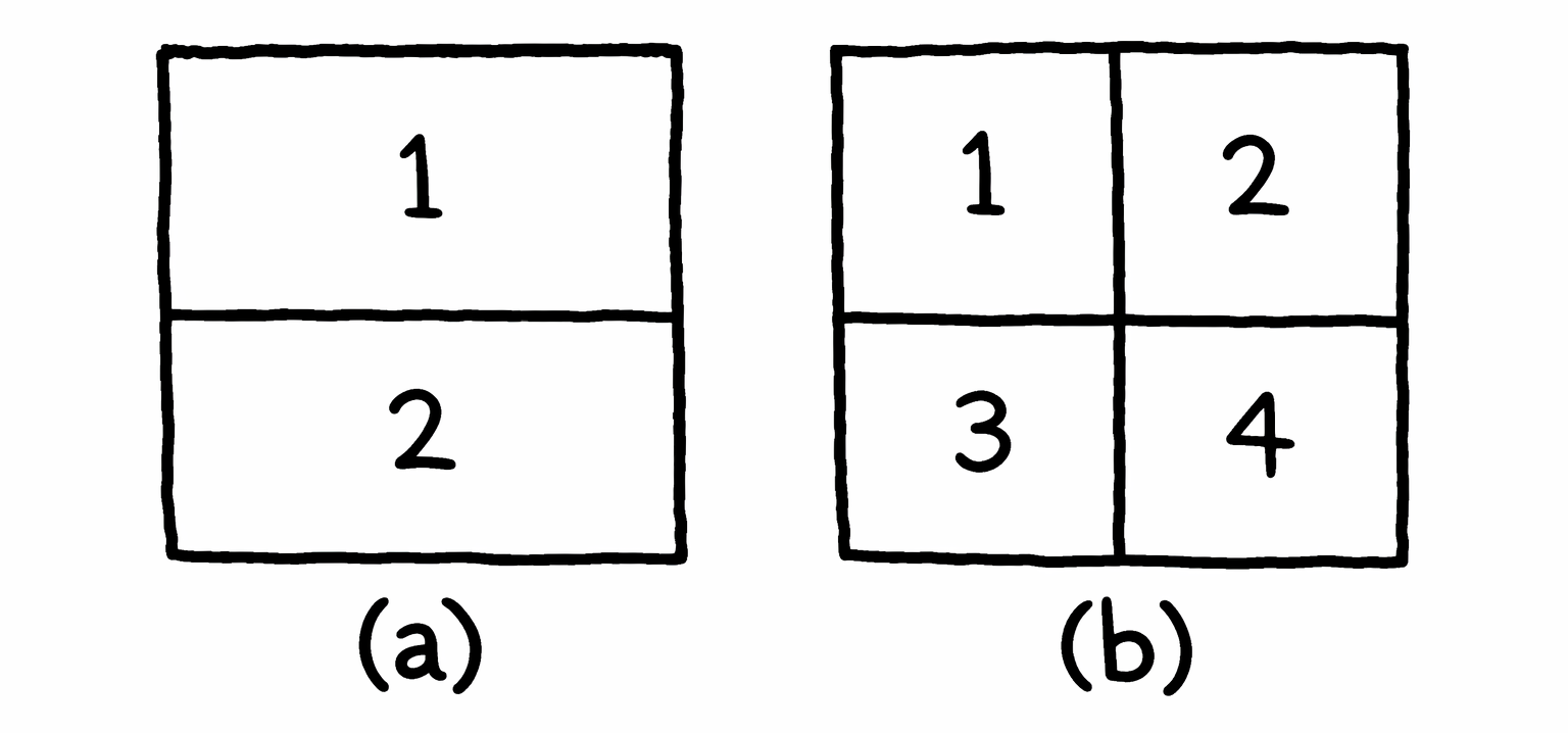
Figure (a): Consider you want to create a language to describe locations in a square. If your language has only two tokens, each token can tell you whether the location is up or down. Now, since there are only two tokens, one bit is sufficient to represent them, making the entropy of this language 1.
Figure (b): Now suppose, if your language has four tokens, each token can give you a more specific location: top-left, top-right, bottom-left, or bottom-right. However, since there are now four tokens, you need two bits to represent them, making the entropy of this language 2.
Hence we can say, entropy calculates how difficult it is to predict what comes next in a language. The lower a language’s entropy, i.e., the lesser the information a token carries, the more predictable that language.
In the example discussed above, the language with only two tokens is easier to predict since you have to predict from only two possible tokens compared to four in the case of the second language.
Hence we can conclude, entropy is highest when outcomes are equally likely and lowest when outcomes are deterministic. Thus, in language modeling:
- A highly structured domain (HTML, SQL, JSON) has lower entropy.
- Casual conversation or creative texts have higher entropy.
Cross entropy
When we train a language model on some data, the goal is to get the model to learn the distribution of the training data. A language model’s cross entropy on a dataset measures how difficult it is for the language model to predict what comes next in this data.
So if $P$ is the true distribution of the training data and $Q$ is the distribution learned by the language model, the cross-entropy $H(P,Q)$ is expressed mathematically as:
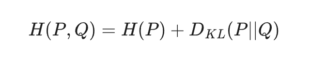
where, $H(P)$ is entropy of training data and $D_{KL}$ represents the Kullback-Leibler divergence, measuring how the learned distribution diverges from the true distribution.
Quick note for those who might not know:
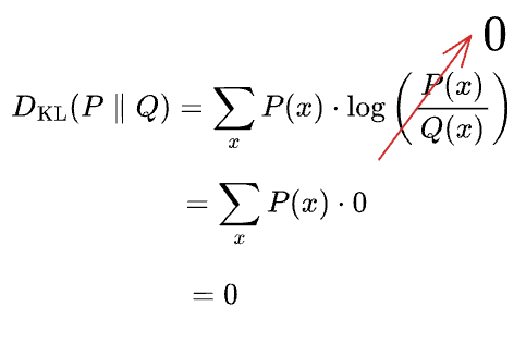
KL divergence is calculated as follows:
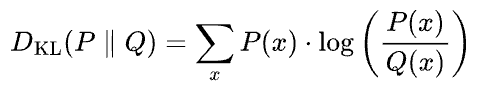
It measures the expected extra information required to encode samples drawn from the true distribution $P$ when using an approximating distribution $Q$. In simple terms, it quantifies how inefficient $Q$ is at representing $P$.
Imagine this. Say $P$ and $Q$ were identical. This should result in zero inefficiency:
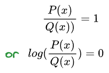
And, hence:
Implication: A language model cannot achieve a cross-entropy lower than the inherent entropy of the dataset ($H(P)$). This is the theoretical lower bound of performance.
A language model is trained to minimize its cross entropy with respect to the training data.
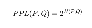
Perplexity
Perplexity (PPL) is the exponentiated cross-entropy, representing the model's absolute uncertainty when predicting the next token. If measured in bits (base 2):
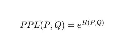
Popular ML frameworks (TensorFlow, PyTorch, etc.), use natural log, making perplexity the exponential of $e$:
A lower perplexity value indicates that the model assigns a higher probability to the true token sequence, or we can also say, the more the uncertainty the model has in predicting what comes next in a given dataset, the higher the perplexity.
With this we have understood about the intrinsic metrics, now let's go ahead and take a look at deterministic evaluation methods.