Building Blocks of LLMs: Decoding, Generation Parameters, and the LLM Application Lifecycle

Recap

Before we dive into Part 4, let’s briefly recap what we covered in the previous chapter.

In Part 3, we moved beyond the foundational translation layer of tokenization and embeddings, and stepped into the core mechanism that actually drives the intelligence, particularly attention.

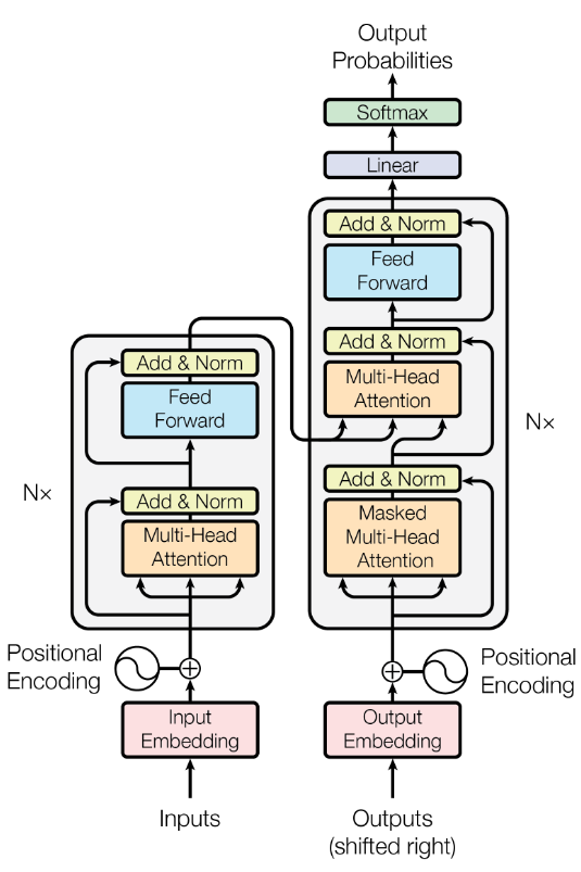
We began by introducing the attention mechanism, the central innovation behind transformers. We explored self-attention in detail. We broke down how input embeddings are projected into Query, Key, and Value vectors, and how scaled dot-product attention computes relevance scores between tokens.

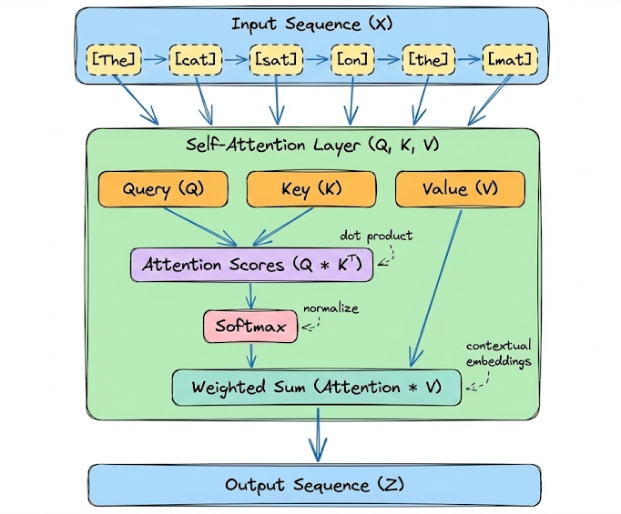
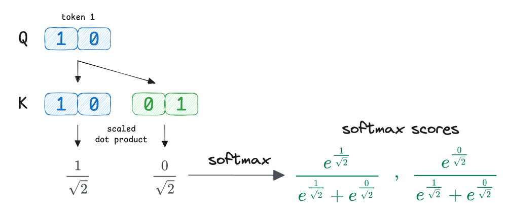
To make this concrete, we also walked through a small illustrative example with manually defined $Q$, $K$, and $V$ vectors.

We then extended the discussion to multi-head attention and saw why a single attention computation is insufficient to capture the many parallel relationships present in language, and how splitting the embedding space into multiple subspaces allows different heads to focus on different aspects.

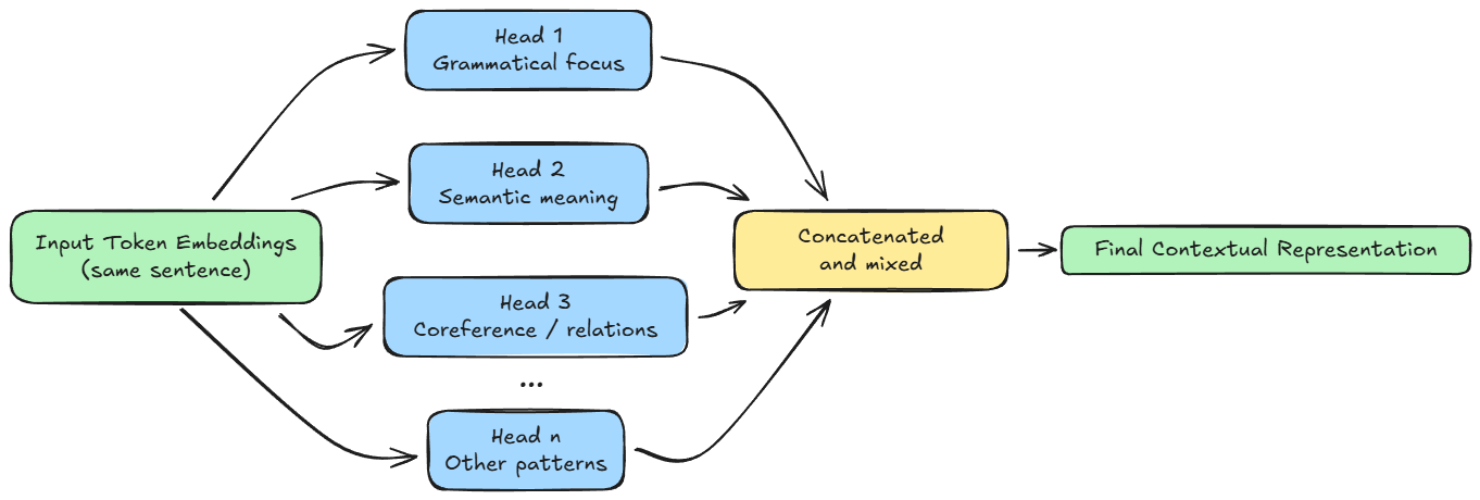
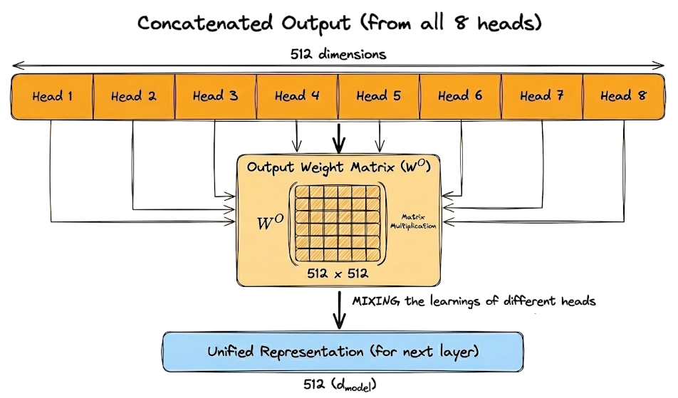
We also examined how head outputs are concatenated and why the final output projection matrix $W^O$ is necessary to recombine and mix information across heads.

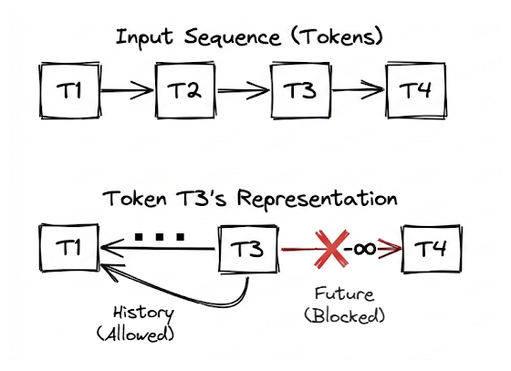
Next, we introduced causal masking, a critical concept for autoregressive language models. We explained why models must be prevented from attending to future tokens during training, and how this is enforced by adding an upper-triangular mask of negative infinity values before the softmax operation.

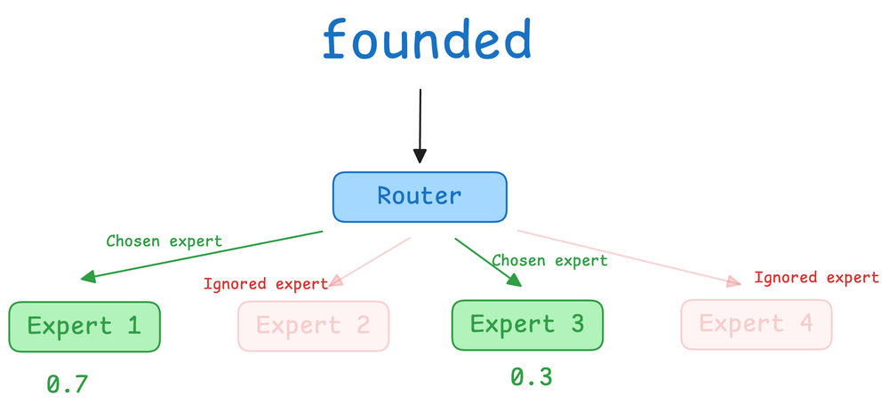
After covering attention, we broadened our perspective to architectural choices. We contrasted dense transformer architecture with mixture-of-experts (MoE) models, explaining how MoE introduces sparse activation through expert selection.

We then shifted from architecture to learning dynamics by examining pretraining and fine-tuning. Pretraining was portrayed as learning the statistical distribution of language via next-token prediction at massive scale, producing a capable but indifferent model.

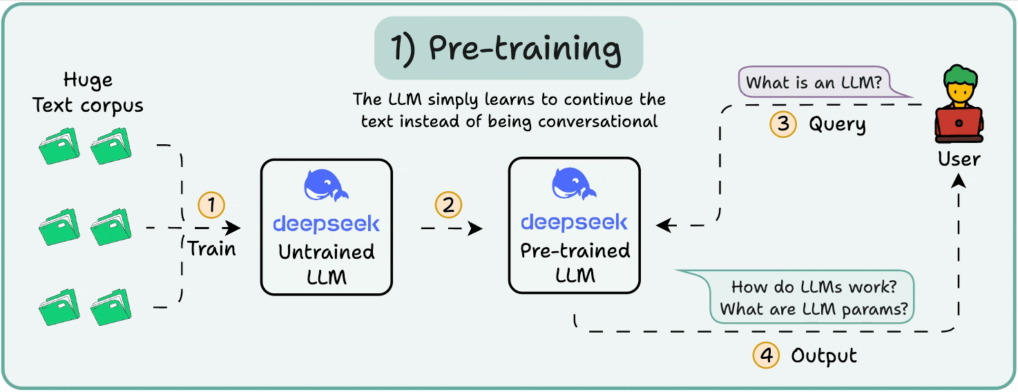
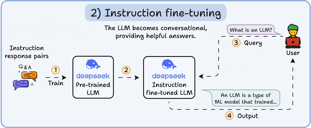
Fine-tuning, particularly instruction tuning, was presented as behavioral conditioning that reshapes this distribution, making the model cooperative, task-aware, and aligned with user intent.

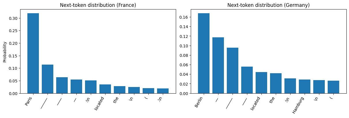
Finally, we grounded these ideas with hands-on experiments. We inspected next-token probability distributions to show that model outputs are fundamentally probabilistic, and that even a single-word change in a prompt can reshape the distribution.

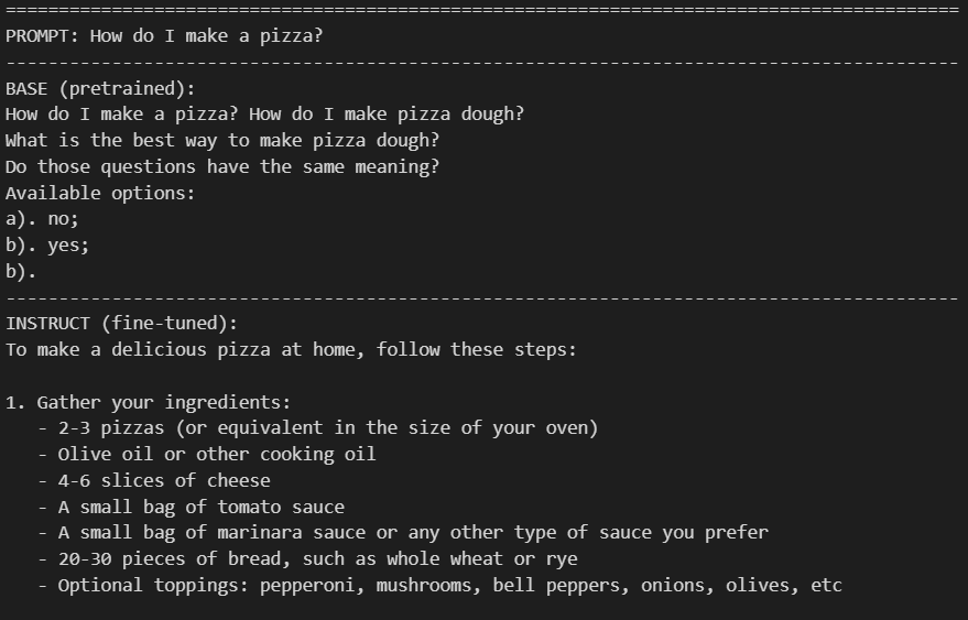
We also directly compared pretrained and instruction-tuned models under identical prompts, clearly demonstrating the difference between text completion and instruction-following behavior.

By the end of Part 3, we had developed a clear understanding of how tokens exchange information, how architectural choices affect efficiency and behavior, and why pretraining and fine-tuning lead to different model personalities.

If you haven’t yet gone through Part 3, we strongly recommend reviewing it first, as it lays the conceptual groundwork for everything that follows.

Read it here:

Building Blocks of LLMs: Attention, Architectural Designs and Training

LLMOps Part 3: A focused look at the core ideas behind attention mechanism, transformer and mixture-of-experts architectures, and model pretraining and fine-tuning.

Daily Dose of Data ScienceAvi Chawla

In this chapter, we will be exploring decoding strategies, generation parameters, and the broader lifecycle of LLM-based applications.

As always, every notion will be explained through clear examples and walkthroughs to develop a solid understanding.

Let’s begin!

LLM decoding

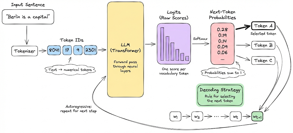
There is a common misconception that large language models directly produce text. In reality, they do not generate text outright. Instead, at each step, they compute logits, which are scores assigned to every token in the model’s vocabulary. These logits are then converted into probabilities using the softmax function.

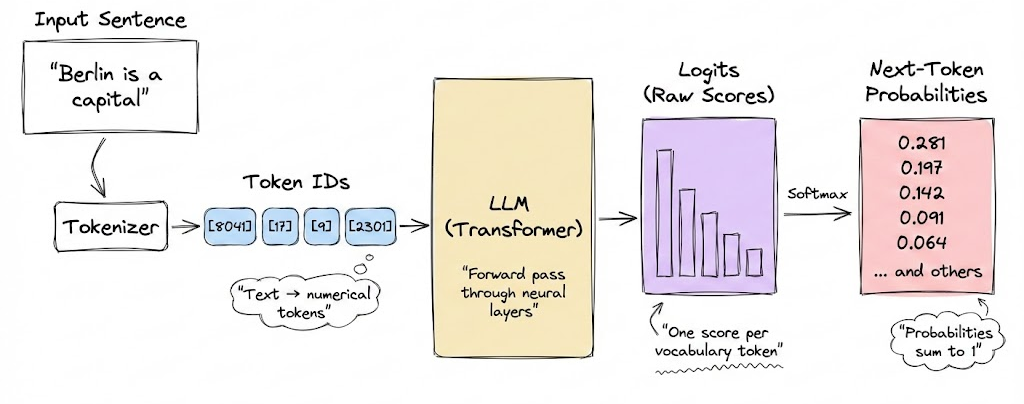
As we saw in the hands-on section of the previous chapter, given a sequence of tokens, each possible next token has an associated probability of being selected. However, how the actual choice of the next token is made has not been discussed by us so far.

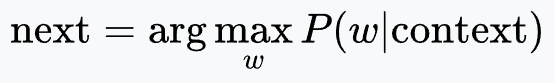
Large language models that are autoregressive predict the next token based on all previously generated tokens. Consider a sequence of tokens $w = w_1, w_2, \ldots, w_t$. The joint probability of the entire sequence can be factorized using the chain rule of probability as:

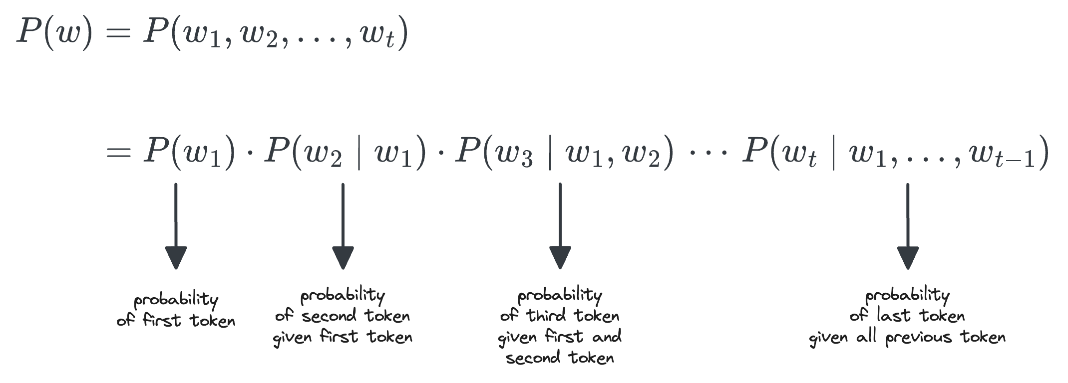
For each token $w_i$, the term $P(w_i \mid w_1, \ldots, w_{i-1})$ represents the conditional probability of that token given the preceding context. At every generation step, the model computes this conditional probability for every token in its vocabulary.

This naturally leads to an important question: how do we use these probabilities to actually generate text?

This is where decoding strategies come into play. Decoding strategies define how a single token is selected from the probability distribution at each step.

Fundamentally, decoding is the process of converting the model’s raw numerical outputs into human-readable text.

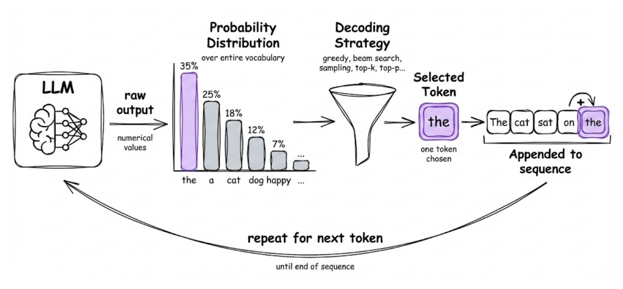
While the model provides a probability distribution over the entire vocabulary, the decoding strategy determines which specific token is chosen and appended to the sequence before moving on to the next step.

How LLM decoding works (in simple language)?

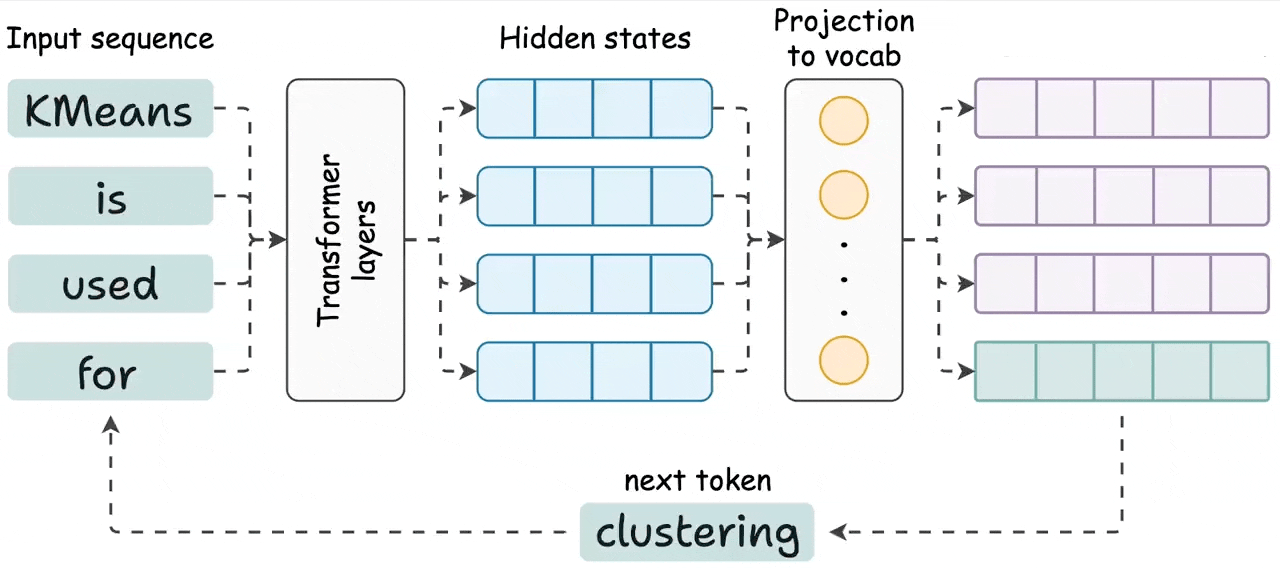
As we already know by now, at its core, an LLM is a next-token predictor that, given a sequence of words or sub-words (tokens), calculates possibilities over its entire vocabulary for what the next most likely token should be.

Decoding strategies are the set of rules used to translate these raw probabilities into coherent, human-readable text by selecting a token. The process is autoregressive: each newly chosen token is added to the sequence and used as part of the input for predicting the subsequent token, continuing until a stopping condition (like an "end-of-sequence" token or maximum length) is met.

Decoding strategies

Now that we know the fundamental meaning of decoding, let's go ahead and discuss the four major decoding strategies themselves. These strategies define how the next token is chosen at each step. We will explain each and compare their behavior:

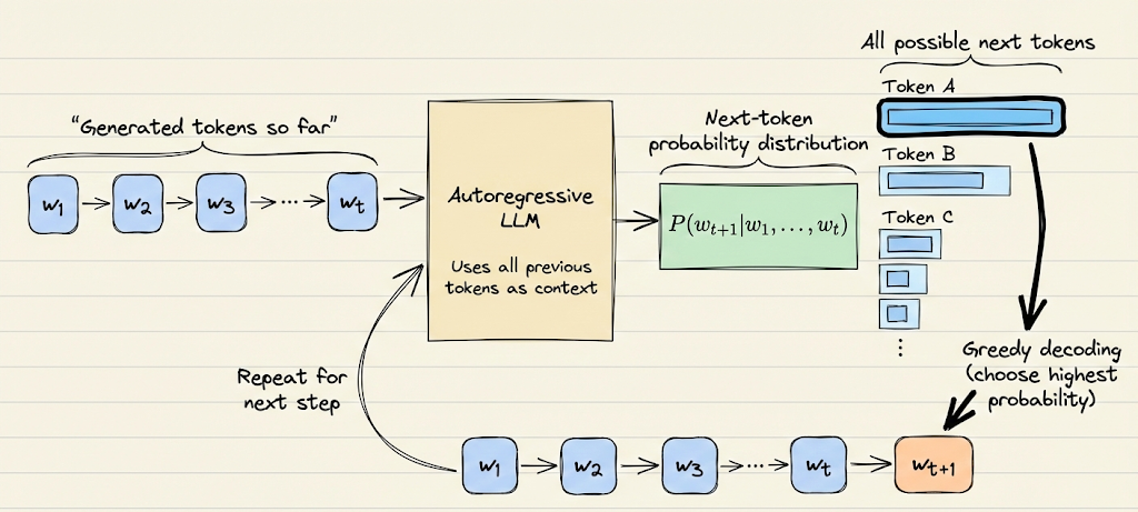
Greedy decoding

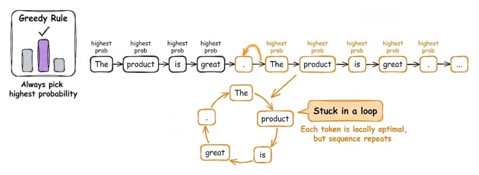
Greedy decoding always picks the highest probability token at each step:

It’s simple and fast (no extra search). The advantage is that it produces the single most likely sequence according to the model’s learned distribution (or at least a local optimum of that).

However, greedy outputs often suffer from repetition or blandness. This is especially true for open-ended generation, where the model’s distribution has a long tail.

For example, a model can get stuck repeating some statement because the model keeps choosing the highest probability continuation, which might circle back to a previous phrase.

Greedy decoding can be appropriate in more constrained tasks.

For instance, in translation, greedy often does well for language pairs with monotonic alignment, and it’s used in real-time systems due to speed. But for tasks like dialog or storytelling, greedy is usually not what you want if you expect diverse and engaging outputs.

Beam search

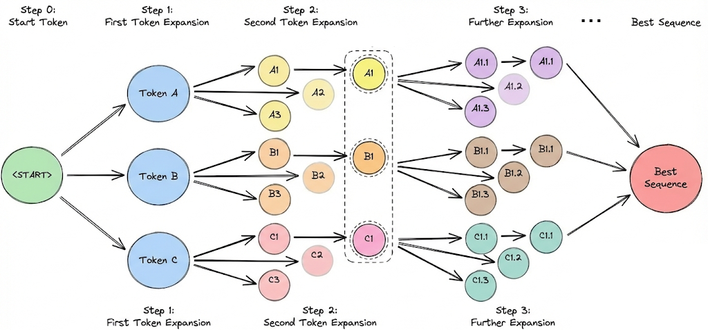
Beam search is an extension of greedy search that keeps track of multiple hypotheses (paths) at each step instead of one.

If beam width is $B$, it will explore the top $B$ tokens for the first word, then for each of those, explore top $B$ for the second word (so $B^2$ combinations, but it keeps only the top B sequences by total probability), and so on.

In essence, beam search tries to approximate the globally most likely sequence under the model, rather than making greedy local choices. This often yields better results in tasks where the model’s probability correlates with quality (like translation or summarization).

However, beam search has known downsides for LLMs in open generation:

• It tends to produce repetitive outputs too (the model maximizing probability often means it finds a loop it likes). In fact, beam search can be worse than greedy search for repetition. It has been observed that beyond a certain beam size, the output quality significantly decreases for storytelling tasks.
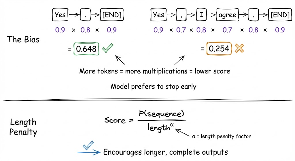
• Beam search can result in length bias: the model often assigns a higher probability to shorter sequences (since each additional token multiplies probabilities, lowering it). Without a length penalty, beam search may prefer ending early to get a higher average score. This is why a length penalty is introduced to encourage longer outputs when appropriate.

In practice, beam search is favored in tasks where precision and logical consistency trump creativity, for example, in summarization (you want the most likely fluent summary), translation, or generating code (where randomness could introduce errors). Meanwhile, for conversational AI or creative generation, beam search can make the model too rigid and prone to generic responses, so sampling is preferred.

Top-K sampling

We will discuss the top-K and top-P parameters in a later section. For now, it’s enough to understand that with top-K sampling, at each generation step, the model samples from at most the top K most probable options.

It's a simple truncation: the low-probability tail is cut off. This avoids weird tokens but still leaves randomness among the top tokens.

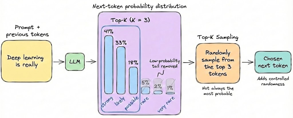
Note that if K is large (e.g. K = 100 or so), it’s almost like full sampling except excluding really unlikely picks, which hardly changes the distribution. If K is very small (e.g. K = 2 or 3), the model becomes only a bit random, it’s like “restricted sampling” where it might alternate between a couple of likely continuations, leading to some limited variation but not a lot.

This type of strategy tends to improve output quality and coherence because low-probability tokens often are low for a reason (either they are nonsensical in context or extremely rare completions). As a result, top-K sampling can reduce the chance of nonsensical completions while still allowing the model to surprise us by not always picking the top option.

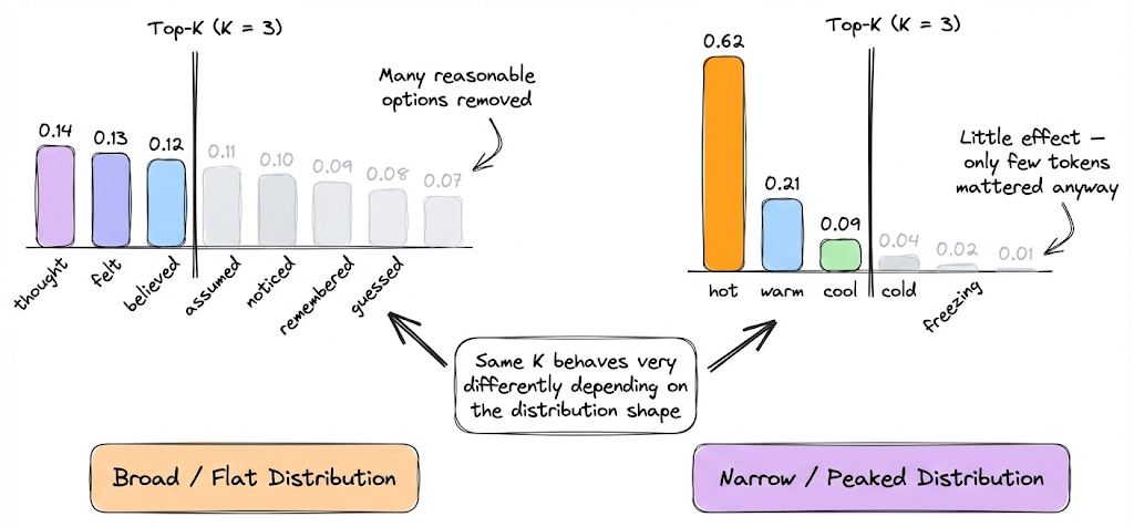
However, like every strategy, there are certain gray areas here too. One drawback is that choosing K is not obvious. A fixed K might be too high in some contexts and too low in others. For example, if the model is very sure about the next word (distribution is peaked), then whether K = 500 or K = 5 doesn’t matter because maybe only 3 tokens had significant probability anyway. But if the distribution is flat (lots of possibilities), limiting to K might prematurely cut off some plausible options.

Despite the above limitation, top-K is computationally efficient and easy to implement, so it’s quite popular.

Nucleus sampling

Nucleus (top-P) sampling includes the smallest set of possible tokens whose cumulative probability is greater than or equal to P.

Nucleus sampling addresses the adaptiveness issue. With top-P, you might sample from 2 tokens in one case (if the model is confident) or 20 in another (if unsure), whatever number is needed to reach the cumulative probability P.

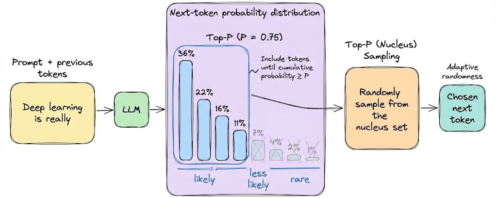
This ensures that the tail is cut off based on significance, not an arbitrary count. So in general, top-P tends to preserve more contextually appropriate diversity. If a model is 90% sure about something, top-P = 0.9 will basically become greedy (only that token considered). If a model is very uncertain, top-P=0.9 might allow many options, reflecting genuine ambiguity.

The quality of top-P outputs is often very good for conversational and creative tasks. It was shown to produce fluent text with less likelihood of incoherence compared to unfiltered random sampling.

That said, one still needs to be reasonable about the choice of P (too high P, like 0.99, brings back long-tail weirdness; too low P, like 0.7, might cut off some normal continuations).

Min-p sampling

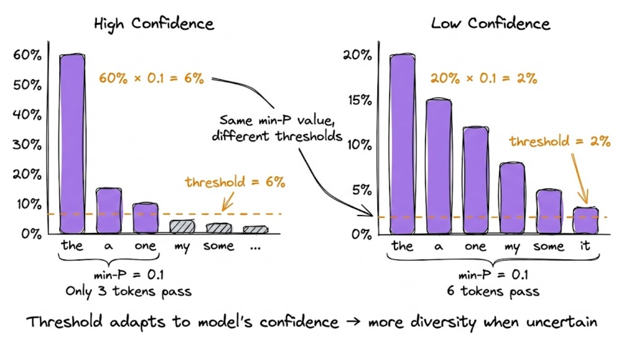
Min-P sampling is a dynamic truncation method that adjusts the sampling threshold based on the model's confidence at each decoding step.

Unlike top-P, which uses a fixed cumulative probability threshold, min-P looks at the probability of the most likely token and only keeps tokens that are at least a certain fraction (the min-P value) as likely.

So if your top token has 60% probability and min-P is set to 0.1, only tokens with at least 6% probability make the cut. But if the top token is just 20% confident, then the adapted 2% threshold lets many more candidates through.