Building Blocks of LLMs: Attention, Architectural Designs and Training

Recap

Before we dive into Part 3, let’s briefly recap what we covered in the previous part of this course.

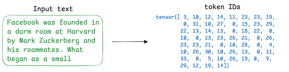
In Part 2, we started with our exploration of the concepts and the core building blocks of large language models. We began by understanding the fundamental concept behind tokenization.

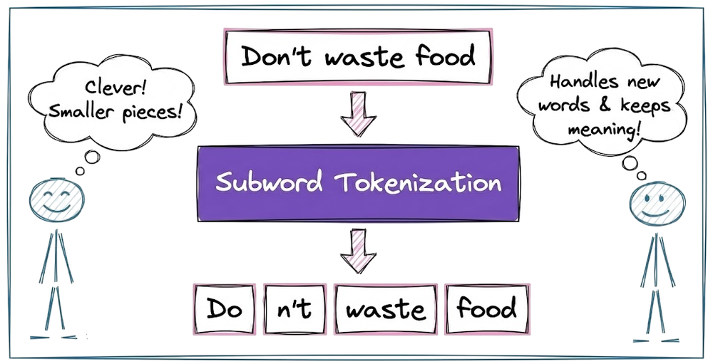
Next, we discussed subword tokenization and understood why it is superior to word-level or character-level tokenization.

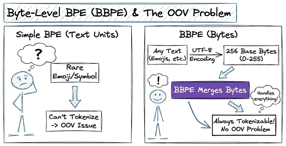
After that, we explored the three most common subword-based tokenization algorithms: byte-pair encoding, WordPiece algorithm and Unigram tokenization. We also learned about the byte-level BPE and understood how it helps in solving the OOV problem.

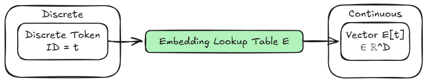
After tokenization, we examined and explored the concept of embeddings and why they are required. We also understood that tokenization is one stage of the two-stage critical translation process, with the other stage being embedding, which maps the tokens into a continuous vector space.

Moving forward, we explored the types of embeddings: token embeddings and positional embeddings. We understood that token embeddings are learned representations that map token IDs to vectors, and positional embeddings inject position information.

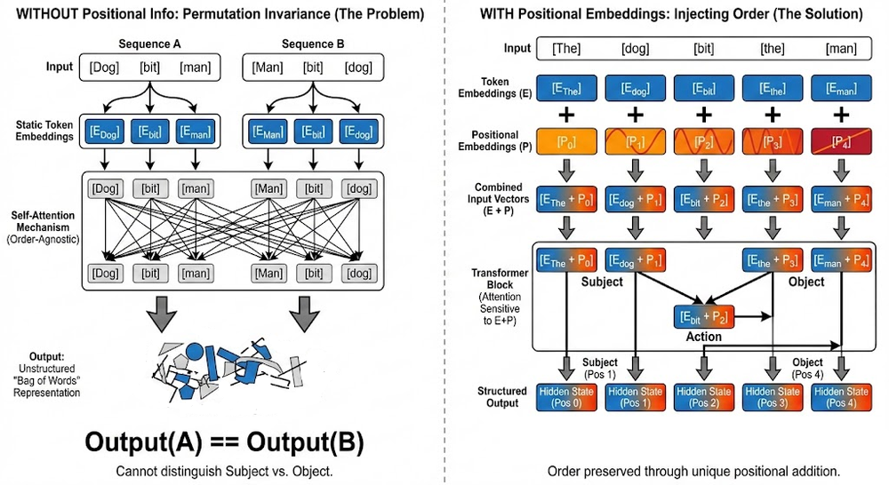
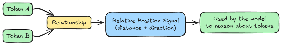
Next, we examined and learned about the two types of positional embeddings: absolute positional embeddings and relative positional embeddings.

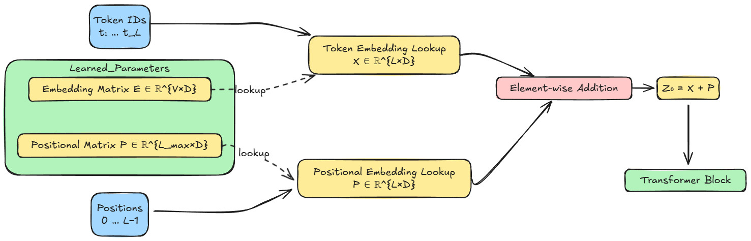
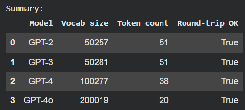
Finally, we took a hands-on approach to tokenization and embeddings. We compared different GPT tokenizers and examined how token embeddings function as a lookup table.

By the end of Part 2, we had a clear understanding of the two-stage translation process. Tokenization converts raw text into discrete symbols drawn from a finite vocabulary, while embeddings convert those symbols into continuous vector representations that neural networks operate on.

If you haven’t yet studied Part 2, we strongly recommend reviewing it first, as it establishes the conceptual foundation essential for understanding the material we’re about to cover.

Read it here:

Building Blocks of LLMs: Tokenization and Embeddings

LLMOps Part 2: A detailed walkthrough of tokenization, embeddings, and positional representations, building the foundational translation layer that enables LLMs to process and reason over text.

Daily Dose of Data ScienceAvi Chawla

In this chapter, we shall further examine key components of large language models, focusing on the attention mechanism, the core differences between transformer and mixture-of-experts architectures, and the fundamentals of pretraining and fine-tuning.

As always, every notion will be explained through clear examples and walkthroughs to develop a solid understanding.

Let’s begin!

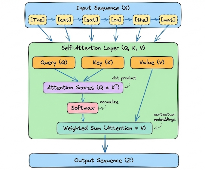
Attention mechanism

“Attention” is the key innovation that enabled Transformers to leapfrog previous RNN-based models. At a high level, an attention mechanism lets a model dynamically weight the influence of other tokens when encoding a given token.

In other words, the model can attend to relevant parts of the sequence as it processes each position. Instead of a fixed-size memory, attention provides a flexible lookup: for each token, the model can refer to any other token’s representation to inform itself, with learnable weights indicating how much to use each other token.

Hence, in a nutshell, attention is the mathematical engine that allows the model to route information between tokens, enabling it to model long-range dependencies.

Self-attention

The most common form of attention is self-attention (specifically scaled dot-product self-attention). In self-attention, each position in the sequence sends queries and keys to every other position and receives back a weighted sum of values.

At its heart, it is a differentiable dictionary lookup. For every token in a sequence, the model projects the input embedding into three distinct vectors, concretely, for each token (at position $i$), the model computes:

• a Query vector $Q_i$​: Represents what the current token is looking for (e.g., a verb looking for its subject).
• a Key vector $K_i$: Represents what the current token "advertises" itself as (e.g., "I am a noun, plural").
• a Value vector $V_i$​: The actual content information the token holds.

Important note:

In a transformer, input token embeddings are linearly projected into Query (Q), Key (K), and Value (V) representations using three separate learned weight matrices.

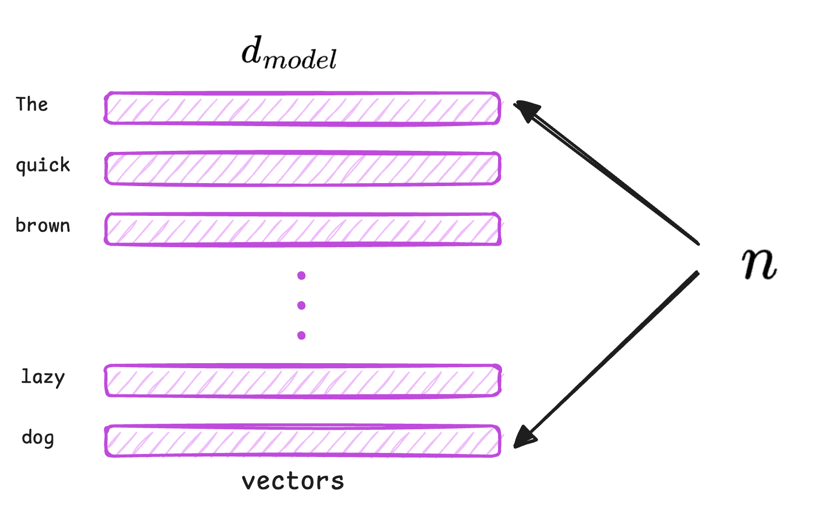
Let the input embedding matrix be: $X \in \mathbb{R}^{n \times d_{\text{model}}}$, where $n$ is the sequence length and $d_{\text{model}}$ is the embedding dimension.

During training, the model learns three distinct weight matrices: $W_Q \in \mathbb{R}^{d_{\text{model}} \times d_k}$, $W_K \in \mathbb{R}^{d_{\text{model}} \times d_k}$ and $W_V \in \mathbb{R}^{d_{\text{model}} \times d_v}$. Here, $d_k$ is the length of a query or key vector and $d_v$ is the length of a value vector.

The Query, Key, and Value matrices are computed as:

• $Q = X W_Q$
• $K = X W_K$
• $V = X W_V$

As mentioned above, $Q_i$, $K_i$ and $V_i$ are all derived from the embedding (or the output of the previous layer) via learned linear transformations. You can think of:

• The Query as the question this token is asking at this layer.
• The Key as the distilled information this token is offering to others.
• The Value as the actual content to be used if this token is attended to.

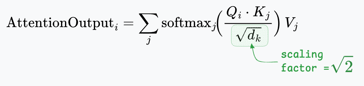
The attention weights between token $i$ and token $j$ are computed as the (scaled) dot product of $Q_i$​ and $K_j$​. Intuitively, this measures how relevant token $j$’s content is to token $i$’s query. All tokens $j$ are considered, and a softmax is applied to these dot products to obtain a nice probability distribution that sums to 1.

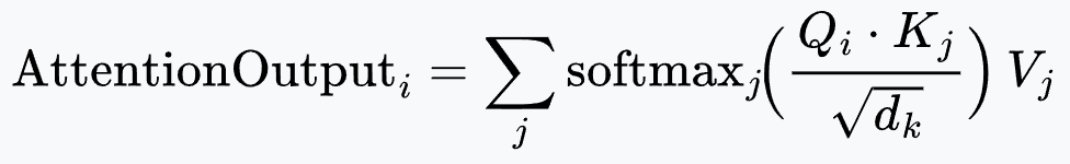
Deconstructing the Formula:

• $Q_i \cdot K_j$: Computes the dot product between the query of token $i$ and the key of token $j$, measuring their relevance.
• $\sqrt{d_k}$ (scaling factor): As the dimensionality $d_k$​ increases, dot-product magnitudes grow, pushing softmax into regions with very small gradients. Dividing by $\sqrt{d_k}$​​ keeps the variance of scores roughly constant and stabilizes training.
• Softmax: Applied over all $j$, it normalizes the attention scores for a fixed query $Q_i$​, producing a distribution of attention weights that sum to 1.
• $V_j$ (Aggregation): The output is a weighted sum of value vectors, producing a context-aware representation for token $i$.

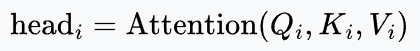
Here's the formula depicted as a diagram:

Dummy example (illustrative)

Now, let's walk through a basic example to understand this better.

Suppose we have a tiny sequence of 2 tokens and a very small vector dimension (2-D for simplicity). We'll manually set some Query/Key/Value vectors to illustrate different attention scenarios:

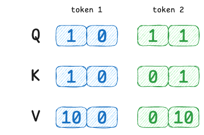
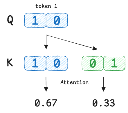
• Token 1 has query $Q_1 = [1,\,0]$
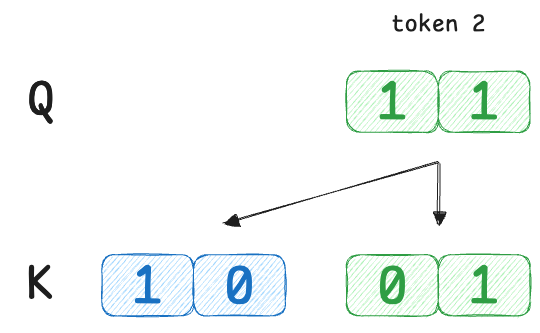
• Token 2 has query $Q_2 = [1,\,1]$
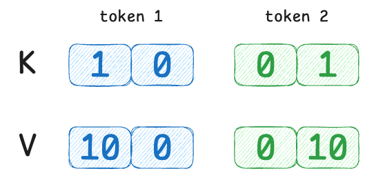
• Token 1’s key $K_1 = [1,\,0]$
• Token 2’s key $K_2 = [0,\,1]$
• Token 1’s value $V_1 = [10,\,0]$
• Token 2’s value $V_2 = [0,\,10]$

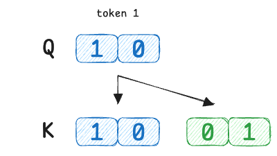
Here, token 1’s query is [1,0] which perfectly matches token 1’s own key [1,0] but is orthogonal to token 2’s key.

Token 2’s query [1,1] is equally similar to both keys. Now we compute attention:

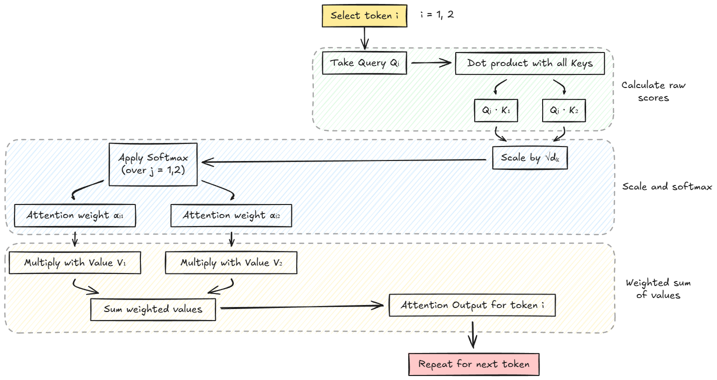
Here is the step-by-step breakdown using the summation formula explicitly for each token index $i$. This method highlights how a single token "looks at" every other token $j$ (including itself) to construct its own output.

Given:

• $d_k = 2$, so scaling factor $\sqrt{d_k} \approx 1.414$.

• Token 1 ($j=1$): $K_1 = [1, 0]$, $V_1 = [10, 0]$
• Token 2 ($j=2$): $K_2 = [0, 1]$, $V_2 = [0, 10]$

Let's compute the attention output for Token 1.

We want to find $\text{AttentionOutput}_1$, which will be a vector that denotes the representation of token 1 based on other tokens.

Thus, we fix $i=1$ and compute attention over all $j$ values → $j=1, 2$.

So the structure of the output is:

Next, we compute raw similarity scores using dot products:

We compare the query of token 1 with every key ($Q_1 \cdot K_j$).

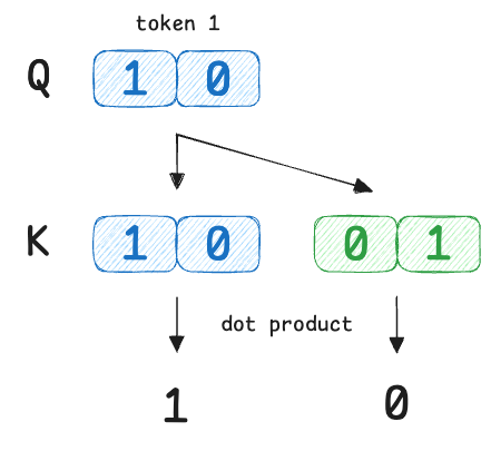
So the raw scores are:

• $s_{1,1}$ = 1
• $s_{1,2}$ = 0

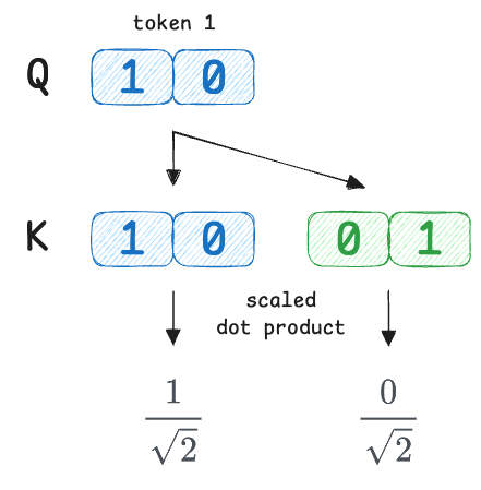
Next, we scale the scores by dividing each score by $\sqrt{2}$:

Moving on, Softmax is applied across the index $j$, while $i$ stays fixed.

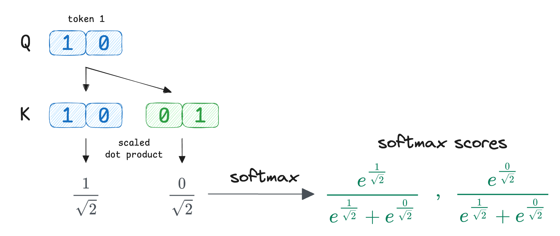
Simplifying the exponential terms, we get the attention scores as:

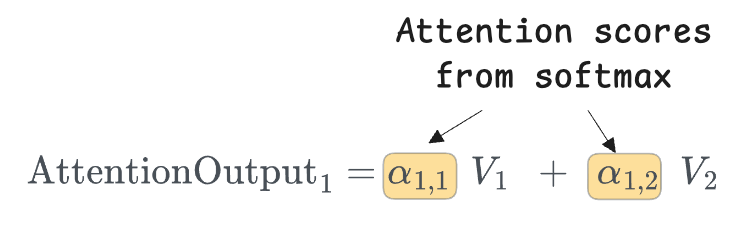
Now we combine the value vectors ($V$) using these attention weights:

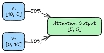
Similar to above, we can find $\text{AttentionOutput}_2$. Consider this as a self-learning exercise, and here are some hints and results for verification:

• We fix $i=2$ and sum over $j=1, 2$.
• Weight $\alpha_{2,1}$ will come out to be: $0.5$
• Weight $\alpha_{2,2}$ will come out to be: $0.5$
• Weighted sum of values: $[5, \, 5]$

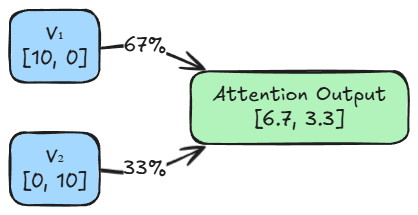
Here's the complete example summarized in the form of a diagram:

Now that we know how the calculations work, let's answer the question, "What does the output actually depict?"

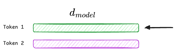
The attention output depicts a contextualized representation of each word based on its relationships (weights) with other words.

For token 1, the attention mechanism calculated weights of 0.67 for itself and 0.33 for token 2. This means the output vector is not just the static definition of $V_1$.

It is a compound concept built from a $67\%$ share of $V_1$ and a $33\%$ share of $V_2$. The model has kept the core identity of the word strong, but has added a slight flavor of the other token.

Similarly, for token 2, the attention mechanism calculated weights of 0.50 for itself and 0.50 for token 1. This means token 2’s representation depends equally on itself and token 1.

In summary, the outputs depict the flow of information. It shows exactly how much context each token absorbed from its neighbors to update its own representation.

With this, we understand the fundamental idea of self-attention. We can now extend this discussion by introducing multi-head attention, which builds on the same principle while enabling the model to capture information from multiple representation subspaces simultaneously.

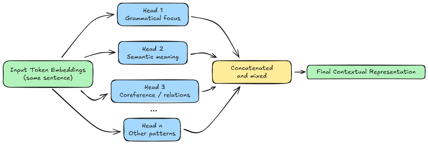
Multi-head attention

In our previous example, we had a single attention mechanism processing the tokens. However, language is too complex for a single calculation to capture everything. A sentence contains grammatical structure, semantic meaning, and references.

To solve this, transformers use multi-head attention (MHA) in practice.

Hence, let's go ahead and understand the conceptual ideas behind multi-head attention.

The dimensionality split

This is where the projection mathematics becomes essential. We take the massive "main highway" of information ($d_{\text{model}}$) and split it into smaller "side roads" (subspaces).

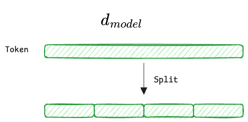
• $d_{\text{model}}$ (the full embedding): Each input token starts as a vector $X \in \mathbb{R}^{d_{\text{model}}}$ (e.g., 512). This vector contains all token information entangled together.
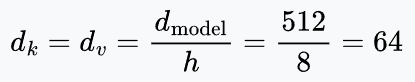
• $h$ (number of heads): We split the workload into $h$ parallel heads (e.g., $h=8$).
• $d_k, d_v$ (the head dimensions): Each head operates on a lower-dimensional subspace. In standard architectures (like GPT/BERT), we divide the dimensions equally, say:

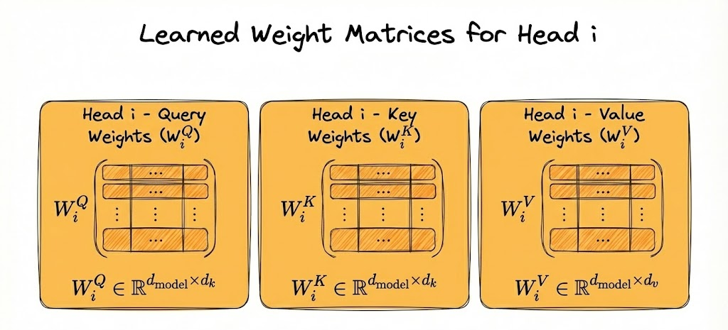
Learnable projections

For each head $i$, the model learns three matrices (which we discussed earlier also):

• $W_i^Q \in \mathbb{R}^{d_{\text{model}} \times d_k}$
• $W_i^K \in \mathbb{R}^{d_{\text{model}} \times d_k}$
• $W_i^V \in \mathbb{R}^{d_{\text{model}} \times d_v}$

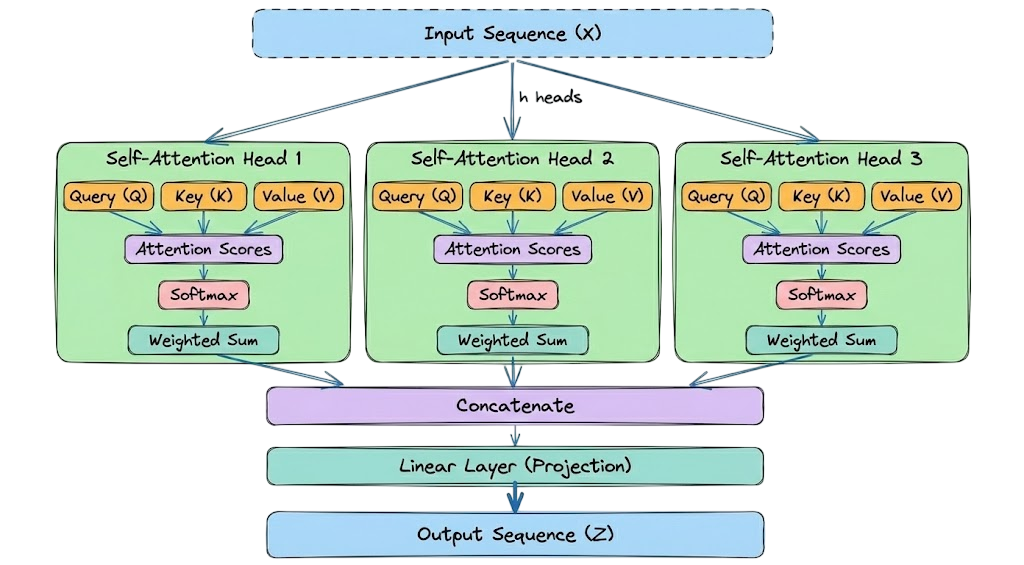
The complete flow

Firstly, the input vector is split into parts, where each part denotes a head:

Each segment of the input goes through the standard attention formula independently, with its own weight matrices:

This results in 8 (total heads) separate vectors, each of size 64.

Next, we stack the output vectors side-by-side to restore the original width.

For example, size: $8 \times 64 = 512$ (Back to $d_{\text{model}}$).

Finally, we multiply by one last matrix, $W^O$.

This $W^O$ (output weight matrix) is the final learnable linear layer in the MHA block. You can think of it as the "manager" of the attention heads.

To understand $W^O$ properly, let's look at the sizes involved:

• As mentioned above, the MHA is the concatenated output of all 8 heads. Size: $8 \text{ heads} \times 64 \text{ ($d_v$)} = 512$ dimensions.
• Desired output: The vector that goes to the next layer (the feed-forward network): $512$ ($d_{\text{model}}$).

Therefore, $W^O$ is a square matrix of size $512 \times 512$.

You might ask: "If the concatenation is already size 512, and we want size 512, why not just stop there? Why multiply by another matrix?"

There's a very critical reason. After concatenation, the vector is segmented:

• Dimensions 0-63: Contain only information from Head 1 (e.g., Grammar).
• Dimensions 64-127: Contain only information from Head 2 (e.g., Vocabulary).
• and so on.

These parts haven't "talked" to each other yet. They are just sitting side-by-side.

Multiplying by $W^O$ allows the model to take a weighted sum across all these segments. It mixes the learnings of different heads to create a unified representation:

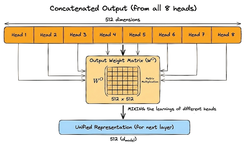
Here is the complete concept in the form of a diagram:

With this, we have completed understanding the key details of multi-head attention (MHA) and attention in general. However, before moving on to another topic, there is one more crucial concept we need to understand: causal masking.

Causal masking

In Generative LLMs (like GPT), we use causal language modeling (CLM), where the objective is to predict the next token.

The Problem: