LLM Inference and Optimization: Fundamentals, Bottlenecks, and Techniques

Recap

In the last chapter (Part 12), we explored how language models can be adapted via fine-tuning.

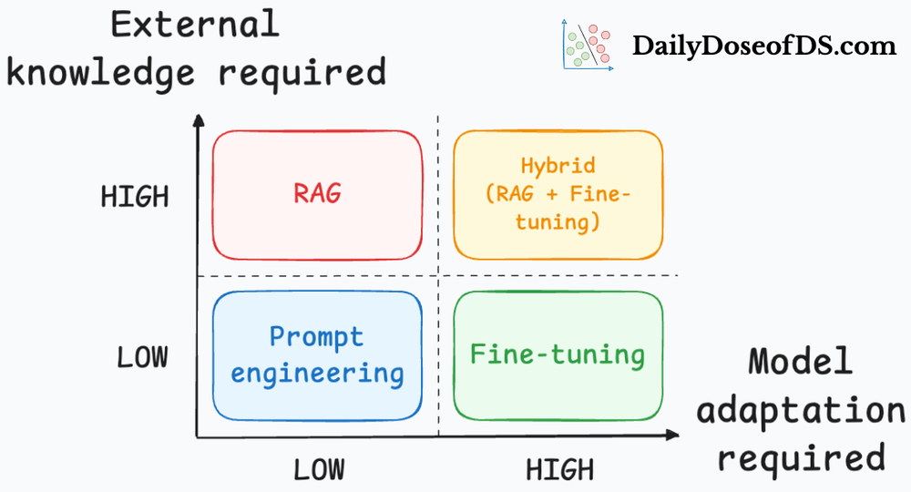
We began by discussing the central question of when fine-tuning is actually worth doing. We studied the reasons to fine-tune and the reasons to avoid it.

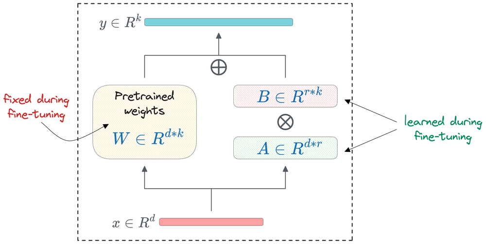
After that, we moved to understanding PEFT techniques. In particular, we explored LoRA and QLoRA. We understood that LoRA reduces the number of trainable parameters, while QLoRA combines ideas of LoRA with quantization.

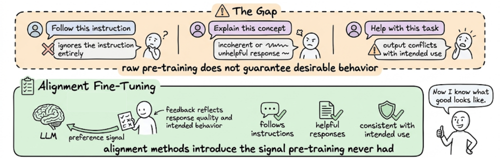
Next, we shifted our focus to alignment fine-tuning. We explored three major preference optimization approaches: RLHF, DPO, and GRPO. Each of these methods provides a different way to push model behavior closer to human preferences or task-specific reward signals.

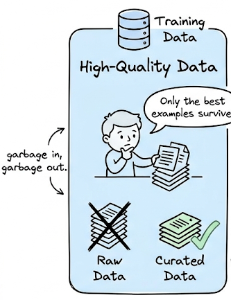
Then, we looked at the role of data in fine-tuning and emphasized the quality and structure of training data.

Finally walked through a hands-on GRPO-based demo using Unsloth, TRL, and the GSM8K dataset.

Overall, the previous chapter established fine-tuning as a tool for adapting LLMs, while also making it clear that it should be used thoughtfully and only when simpler approaches are not enough.

If you haven’t yet gone through Part 12, we recommend reviewing it first, as it helps maintain the natural learning flow of the series.

Read it here:

LLM Fine-tuning: Techniques for Adapting Language Models

LLMOps Part 12: Understanding LLM fine-tuning, parameter-efficient methods like LoRA and QLoRA, and alignment techniques such as RLHF, DPO, and GRPO.

Daily Dose of Data ScienceAvi Chawla

In this chapter, we will be exploring LLM inference and optimization. We will understand how inference works and what techniques are used to optimize it.

As always, every notion will be explained through clear examples and walkthroughs to develop a solid understanding.

Let’s begin!

Key throughput and latency metrics

Understanding and optimizing inference without understanding the right metrics is probably not a very smart thing to do. Thus, let’s first establish how we measure LLM inference performance in the first place:

• Time to first token (TTFT): The time taken to generate the first token after sending a request. It basically evaluates how fast the model can start responding. Think of TTFT as the startup latency for a query.
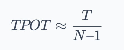
• Time per output token (TPOT): Once the first token is out, TPOT measures the steady-state speed of generation: the average time to produce each subsequent token. A lower TPOT means the model can produce tokens faster, leading to higher tokens per second. Formally, if an output has $N$ tokens and the total generation time after the first token is $T$, then:

• End-to-end latency (E2E): The total time from request to receiving the final output token.
• Throughput: How much work the system can handle per unit time. Throughput is often measured in two ways:
  • Requests per second (RPS): tells how many requests can be completed per second.
  • Tokens per second (TPS): measures token processing rate, including input tokens (input TPS) and output tokens (output TPS) across all requests.

• Latency percentiles (p95, p99) capture the tail experience. A system with an average TTFT of 200ms may have a p99 TTFT of 2 seconds, meaning 1% of users wait 10× longer. Thus, our objectives/SLOs should also target p95 or p99, not just averages (especially important if consistency is critical).
• Goodput is the fraction of requests meeting all objective/SLO constraints simultaneously (e.g., TTFT < 500ms AND TPOT < 50ms).

Now that we understand the metrics, let’s go ahead and build a precise mental model of how the LLM inference mechanism works.

How LLM inference works

Autoregressive language models generate tokens one at a time, where each new token depends on all previous tokens. This dependency is the fundamental constraint that makes understanding inference and optimization challenging.

The two phases of LLM inference

Critically, LLM inference isn’t a uniform workload; it has two distinct phases:

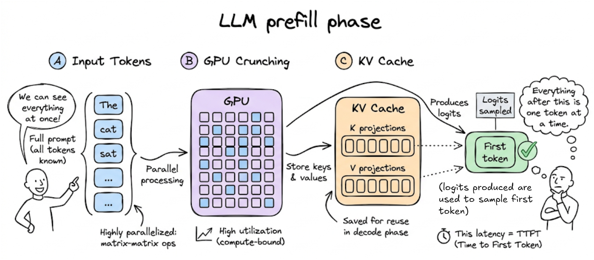
• Prefill phase: The model processes the input tokens to compute the intermediate states (keys and values), which are used to generate the first output token. Because the full extent of the input is known, at a high level, this is a highly parallelized matrix-matrix operation, and the GPU can reach high utilization (the operation is compute-bound). The K and V projections are stored in what we call the KV cache for later reuse (more on it later in the chapter). The prefill phase completes by building the full KV cache for the prompt and producing the logits from which the first output token is sampled. The decode phase then generates subsequent tokens one at a time. The time until this first token is generated maps directly to the TTFT metric and is dominated by the prefill phase.

• Decode phase: The model generates output tokens one by one. At each step, only the single newest token's Q, K, V projections are computed. The new K and V vectors are appended to the KV cache, and the new Q vector attends against all cached K vectors. This results in low-parallel, matrix-vector kind of operations with poor hardware utilization. The arithmetic intensity plummets: tons of memory accesses for a tiny operation. Thus, the decode phase is usually memory-bandwidth-bound and hence maps to the TPOT metric.