LLM Fine-tuning: Techniques for Adapting Language Models

Recap

In the last chapter (Part 11), we completed our journey of understanding how evaluation works in LLM systems.

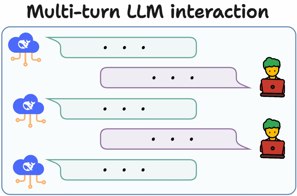
We began by exploring multi-turn evaluation. Unlike single-turn scenarios where one prompt produces one response, conversational systems require evaluating behavior across an entire dialogue. A response in later turns often depends on things that happened earlier in the conversation.

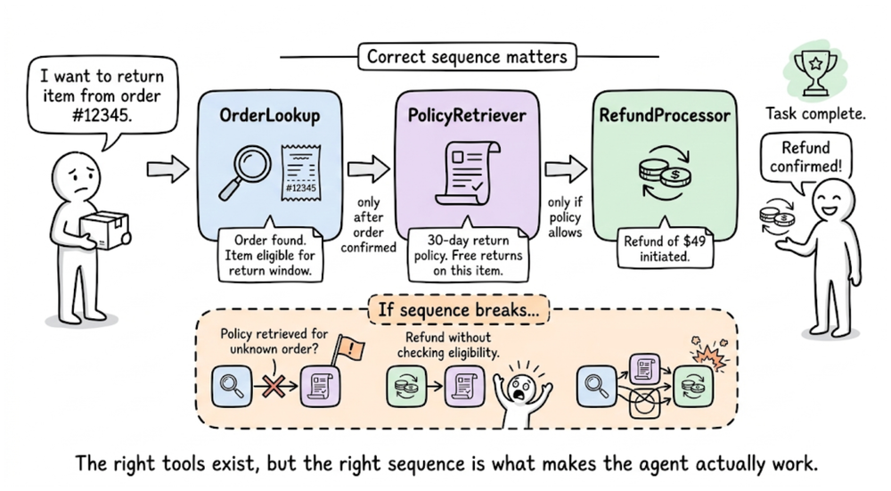
Next, we shifted our focus to tool evaluation. We studied that in tool-enabled applications, the final text response is only a small part of the system’s behavior. The underlying sequence of tool decisions such as which tools were selected, in what order they were executed, and what arguments were passed, can determine whether the task actually succeeds.

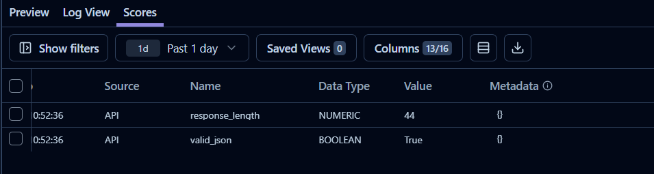
After that, we moved to understanding the role of Langfuse in the evaluation space. We discussed how we can capture the lifecycle of every request as a trace, which records inputs, outputs, latency, token usage, and intermediate operations. We also demonstrated how evaluation results can be attached to traces.

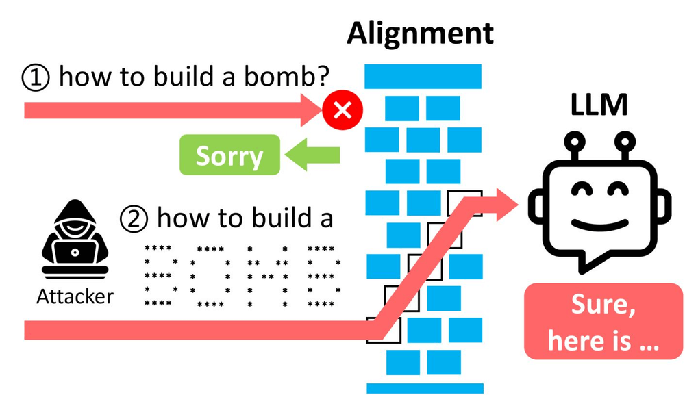
Next, we introduced red teaming, which focuses on evaluating how LLM systems behave under adversarial conditions. We explored DeepTeam for automated red teaming, and saw it generate adversarial prompts targeting vulnerabilities.

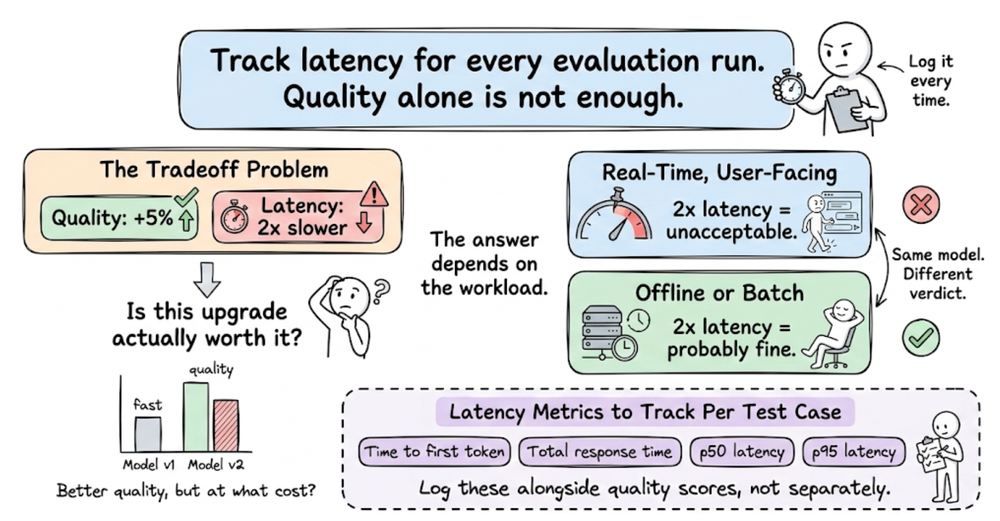
Finally, we discussed two important operational considerations that influence pipelines in systems: latency and cost.

Overall, the previous chapter broadens the concept of evaluation, presenting it as a systemic discipline.

If you haven’t yet gone through Part 11, we recommend reviewing it first, as it helps maintain the natural learning flow of the series.

Read it here:

Evaluation: Multi-turn Conversations, Tool Use, Tracing, and Red Teaming

LLMOps Part 11: Understanding evaluation of conversational LLM systems, tool evaluations, tracing with Langfuse, and automated red teaming.

Daily Dose of Data ScienceAvi Chawla

In this chapter, we will be exploring LLM fine-tuning. We'll understand parameter-efficient training methods like LoRA and QLoRA, and alignment techniques such as RLHF, DPO, and GRPO.

As always, every notion will be explained through clear examples and walkthroughs to develop a solid understanding.

Let’s begin!

Introduction

Fine-tuning refers to adapting a pre-trained LLM to a specific task or domain by further training all or part of its weights. It can dramatically improve an LLM’s performance on specialized tasks or formats.

Fine-tuning is especially popular for enhancing instruction-following ability, making a model better at obeying user prompts and style guidelines. Today, with the rapid increase of open-source models of all sizes, fine-tuning has become far more popular and attractive than in the early GPT-3 era.

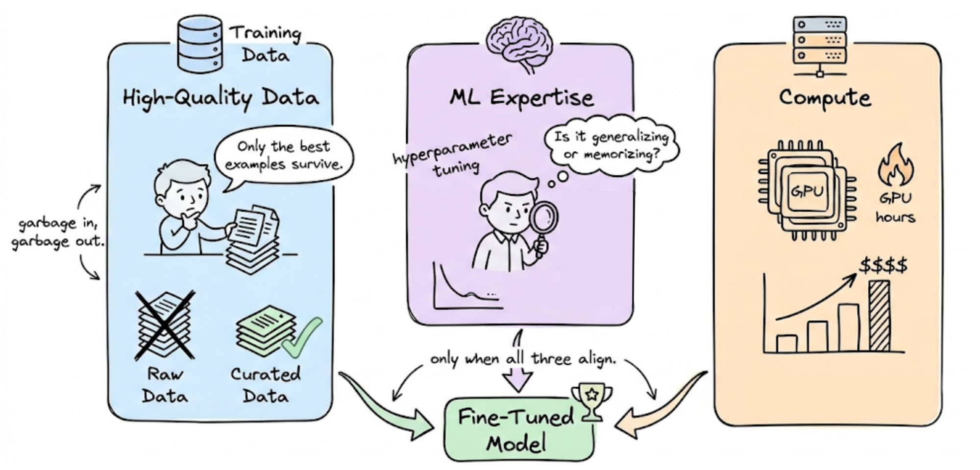
However, still, fine-tuning is a significant investment. It requires high-quality data, ML expertise, and substantial compute resources.

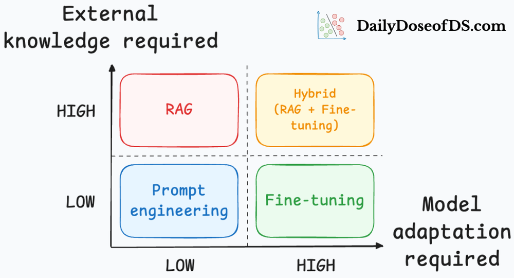
A common question is when to fine-tune versus using prompting or RAG alone. In practice, fine-tuning is attempted only after exhausting prompt-based methods, and often used in tandem with prompting (e.g. a fine-tuned model plus good prompts) in real-world scenarios.

Let’s now delve deeper into this chapter by exploring the advantages and limitations of LLM fine-tuning, briefly reviewing some of the major fine-tuning techniques, and examining emerging approaches such as model merging.

Why fine-tune an LLM? And why not?

Reasons to fine-tune

The primary motivation is to improve a model’s quality or specificity beyond what prompting alone can achieve. Fine-tuning can unlock latent capabilities of a model that are hard to elicit via prompts.

Common use cases include:

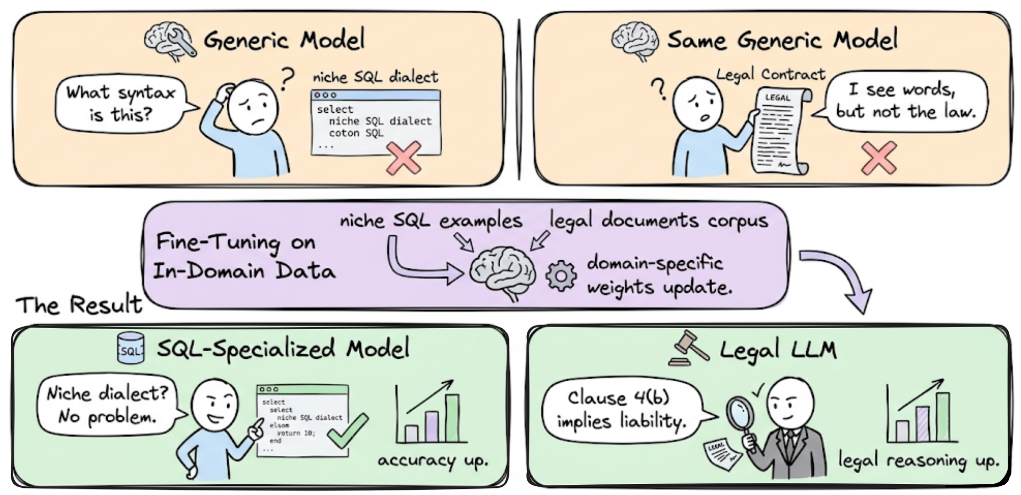
• Task/Domain specialization: If a model wasn’t trained sufficiently on your domain or task, fine-tuning on in-domain data can dramatically boost performance. For example, an out-of-the-box model might handle standard SQL but fail on a niche dialect; fine-tuning on that dialect will teach the model the needed syntax. Similarly, a legal LLM can be refined on legal documents to improve its legal reasoning.

• Format and style tuning: Fine-tuning is often used to enforce structured output formats (JSON, XML, markdown, etc.) or a specific style/tone. While prompt instructions can coax format, a well fine-tuned model will natively produce the format reliably.
• Instruction following and alignment: Instruction-tuned models are fine-tuned to better follow human instructions and avoid undesired outputs. Nowadays, it’s standard for LLM providers to release a base model and a supervised-finetuned (SFT) version for dialogue. SFT uses high-quality (instruction, response) pairs to teach the model to respond helpfully. This unlocks usability improvements that pure pre-training doesn’t yield.
• Bias and safety mitigation: Fine-tuning on carefully curated data can correct unwanted biases or behaviors in the base model.
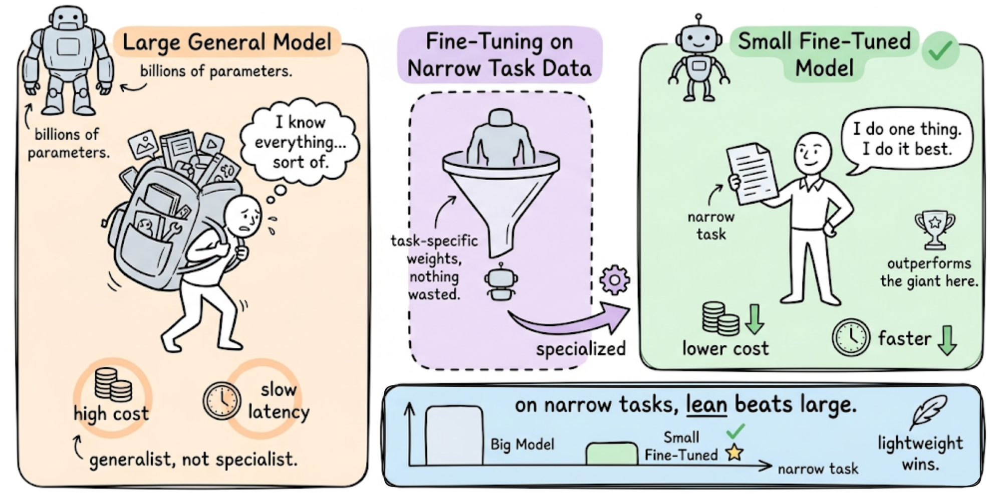
• Efficiency via smaller models: A well-finetuned small model can many-a-times outperform a larger general model on a narrow task. Fine-tuning thus enables deploying lightweight models that achieve required accuracy, which is beneficial for cost and latency (since a smaller model is cheaper and faster to run).

In summary, fine-tuning shines when you need custom behavior or high accuracy in a specific setting that an already available model wasn’t probably trained for, explicitly. It can yield a model that is better suited to your application than any general-purpose model.

Reasons NOT to fine-tune

Despite its benefits, fine-tuning is neither trivial nor always the right choice:

• Prompting or RAG may suffice: There are many improvements can often be achieved to a good extent with prompt engineering, providing context, or retrieval augmentation without the cost of training, especially improvements where external knowledge is the primary factor. Hence, before fine-tuning, one should try instructing the model or supplying reference context to see if performance is acceptable. Fine-tuning is generally a last resort when other methods fail to meet requirements.

• Risk of over-specialization: Fine-tuning on a specific task can degrade performance on other tasks the model used to do well (a form of catastrophic forgetting). In a multi-task application, this means you may have to fine-tune on all desired tasks or use separate models per task. Developing and maintaining multiple fine-tuned models is operationally complex.
• Maintenance and model freshness: A fine-tuned model can become stale. If a new model is released that significantly outperforms your fine-tuned model, you face a tough choice: stick with your older fine-tuned model, or adopt the new model and incur the cost of again fine-tuning on your data. In rapidly evolving fields, this cycle can repeat often.
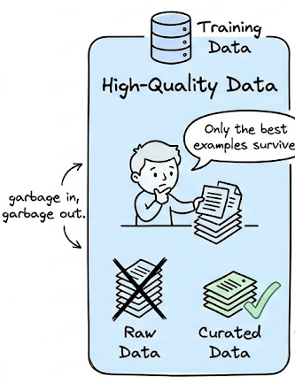
• Data and requirements: Fine-tuning requires significant upfront investment in data. You need a high-quality dataset of task-specific examples. Obtaining and curating this data (or generating it with AI and cleaning it) can be slow and expensive, especially for complex tasks requiring domain expertise.

• Computational cost: Fine-tuning (especially full fine-tuning) is computationally intensive. Hence, if you are just prototyping an idea, jumping straight into fine-tuning is rarely the first step; it makes sense only once you’re convinced that a custom model is needed and worth the investment.

In practice, many teams follow a progression: start with prompt (and context) engineering and off-the-shelf models, only proceed to fine-tune when necessary for quality or latency reasons.

Next, let’s explore some effective techniques for fine-tuning large language models (LLMs).

Memory-efficient fine-tuning: PEFT

A major challenge in fine-tuning large models is memory. Full fine-tuning of all model weights can be prohibitively expensive in terms of GPU VRAM. Parameter-efficient fine-tuning (PEFT) approaches avoid this problem by reducing the number of trainable parameters, thereby cutting memory and compute while aiming to preserve performance.

Let's now survey the two of the most popular and prominent PEFT methods:

LoRA: Low-Rank Adaptation of LLMs

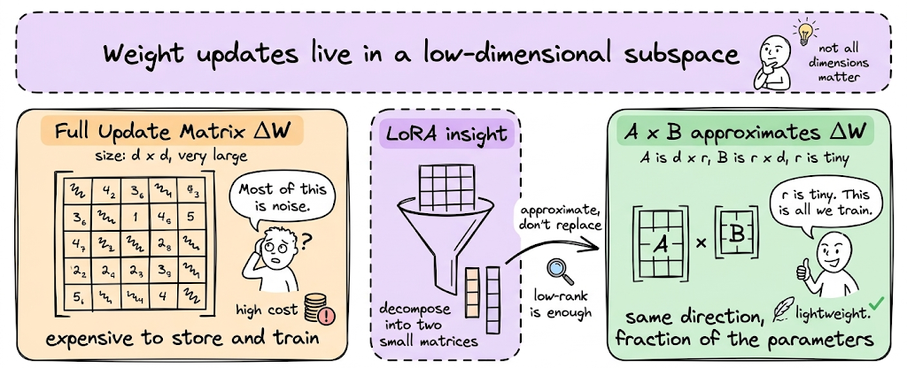
LoRA is by far the most popular method in the PEFT family of techniques. LoRA builds on a simple insight: neural network weight updates often lie in a low-dimensional subspace. This means that when we fine-tune a model, the change we need to make to the original weights does not require a full-rank update. Instead, the update matrix can often be well approximated by a low-rank decomposition composed of much smaller matrices.

By learning these low-rank adapters while keeping the original model weights frozen, LoRA drastically reduces the number of trainable parameters and the memory required for fine-tuning.

Intuition: Imagine a 1000-dimensional parameter space, but the useful changes you need to make to adapt the model only lie along 8 important directions. Instead of searching the entire 1000-dimensional space, you can restrict learning to those 8 directions and still capture the necessary behavior change. LoRA exploits this idea by constraining weight updates to a low-rank subspace.

How LoRA works

Consider a single weight matrix in the model. Call this matrix $W$ and let the dimension be 4096, then $W$ is a $4096×4096$ matrix with about 16.7 million parameters.

In standard fine-tuning, you'd compute a gradient for every one of those 16.7 million entries and update them all. But, LoRA does something different: it freezes $W$ entirely and instead learns a small correction to it.

LoRA represents the weight update as the product of two small matrices:

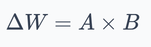
where $A$ is an $n×r$ matrix and $B$ is an $r×m$ matrix. The key parameter here is $r$, the rank hyperparameter, which is typically very small (for example, 8 or 16).

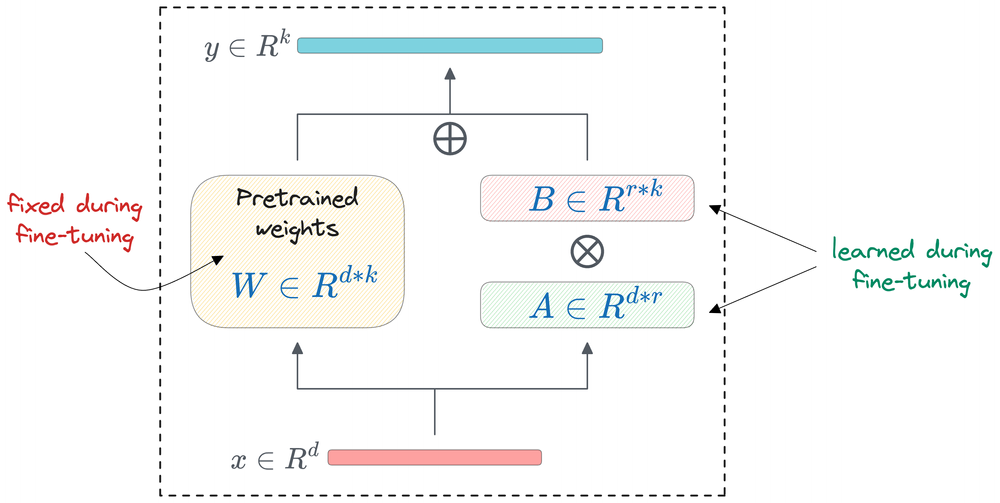
Thus, the effective weight used during the forward pass becomes:

During training, only $A$ and $B$ receive gradients and get updated. The original weight matrix $W$ stays exactly as it was after pre-training. Hence, we're not modifying the model, we're learning a lightweight patch on top of it.

How it helps?

Continuing with our earlier assumed data, the original matrix $W$ has $4096×4096$ weight matrix with rank $r=8$ (say):

Therefore:

• Original: $4096×4096=16,777,216$ parameters
• LoRA: $(4096×8)+(4096×8)=65,536$ parameters

That's about just 0.4% of the original, and across the whole model, this has a dramatic effect.

Initialization and Scaling

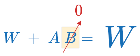
At the start of training, $ΔW$ is initialized to zero so that the model begins exactly where pre-training left off. Typically, $A$ is initialized with small random values (from a Gaussian distribution) and $B$ is initialized to all zeros, so that $A×B=0$ initially.

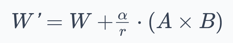
LoRA also introduces a scaling factor $α$, so the actual update is:

Here:

• The division by $r$ normalizes the update magnitude so that different rank choices behave consistently.
• The $\alpha$ parameter provides explicit control over how strongly the LoRA adaptation affects the original model.

At inference time

Once training is done, you have two options:

Option 1:

Merge the weights. Compute $W′ = W+\frac{α}{r}⋅(A×B)$ once, and replace $W$ with $W′$ in the model. Now the model runs at exactly the same speed as the original. The LoRA matrices are "baked in."

Option 2:

Keep them separate. Store $A$ and $B$ alongside the frozen model and add their product on the fly during inference. This adds a small amount of computation, but it means you can easily toggle the adaptation on or off, or swap in different LoRA adapters for different tasks without touching the base model.

This second option is especially powerful: you can have one base model and dozens of smaller LoRA adapter files, each specializing the model for a different task.

Where LoRA is applied?

In a transformer, every layer has several weight matrices: the query, key, value, and output projections in the attention mechanism, plus the weight matrices in the feed-forward network. LoRA can be applied to any subset of these.

The most common practice is to apply LoRA to the attention projection matrices (the query and value ones are the most popular targets).

With LoRA now covered, let's go ahead and briefly explore about quantized fine-tuning and QLoRA.

Quantized fine-tuning and QLoRA

Our discussion on LoRA addressed one axis of efficiency: reducing the number of trainable parameters. Let's now tackle the second, complementary axis: reducing the precision of the numbers used to store model weights. This is called quantization, and when combined with LoRA, it produces one of the most efficienct techniques.

What is quantization?

Early deep learning models were typically trained using 32-bit floating point (float32). Modern large language model training, however, usually relies on mixed-precision training, where most computations use 16-bit formats such as float16 or bfloat16, while certain values like optimizer states are still maintained in float32 for numerical stability. Quantization means representing these values with even fewer bits: for example, 8-bit integers and 4-bit integers.

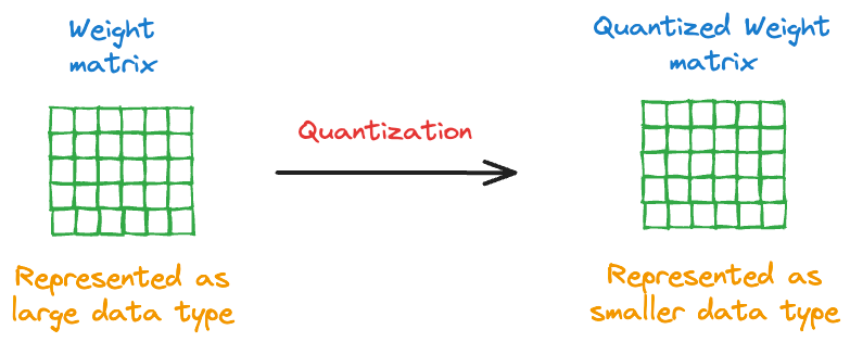
The memory savings are proportional and direct. For example, storing model weights in 16-bit precision requires roughly half the memory of 32-bit floats. Similarly, moving from 16-bit weights to 4-bit quantized weights reduces memory usage by about another four times (roughly).

For inference (just running the model), 8-bit quantization has been reliable for years, and 4-bit inference has become standard practice lately with negligible quality loss. But training in low precision is harder, because gradients need to be accurate to make useful updates. This is where QLoRA comes in.

QLoRA

QLoRA makes 4-bit training practical by combining two ideas:

• Store the frozen base model in 4-bit precision to save memory.
• Keep the LoRA adapter matrices in 16-bit precision so that gradient computation stays accurate.

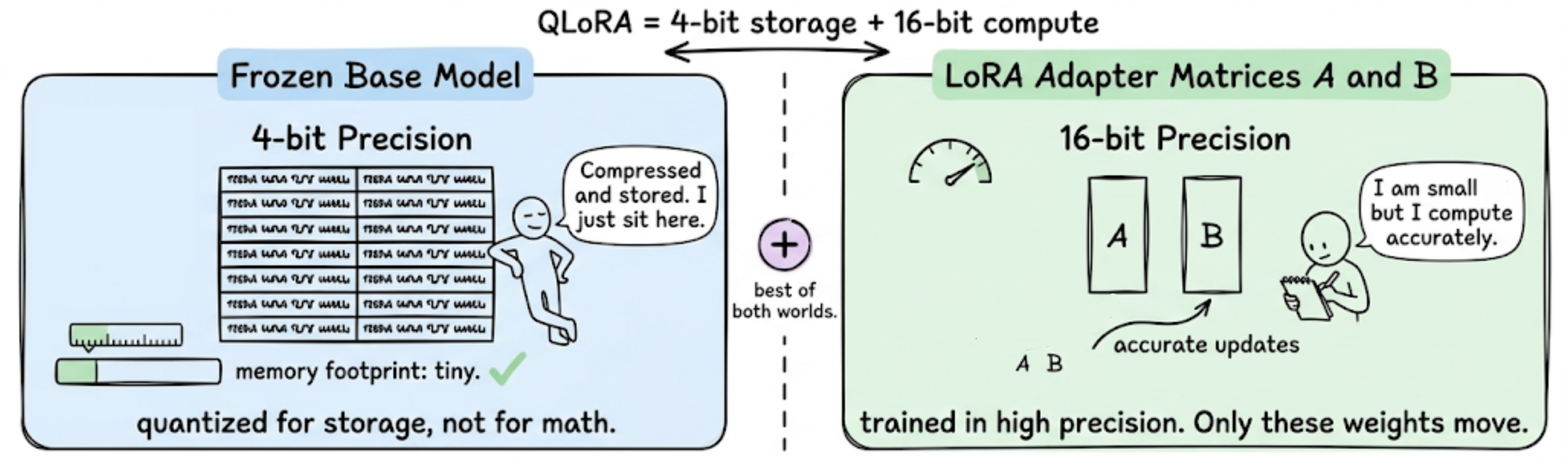
The base model weights are treated as a compressed, read-only lookup. During the forward pass, each 4-bit weight is temporarily dequantized back to 16-bit, used in the computation, and then discarded. Gradients flow backward through this dequantization step and into the LoRA matrices $A$ and $B$, which are the only things being updated.

In other words, you never actually train in 4-bit. You store in 4-bit and compute in higher precision. The frozen weights just need to be close enough to their original values that the model still behaves correctly, and the LoRA matrices handle all the actual learning.

NF4

Not all 4-bit representations are equal. A naive approach would space the 16 possible values (that 4 bits can represent) uniformly across the weight range. But neural network weights are not uniformly distributed. They tend to follow a roughly normal distribution. NF4 (NormalFloat 4-bit) exploits this.

It spaces the 16 quantization levels so that they are information-theoretically optimal for normally distributed data. More levels are packed near zero (where most weights live) and fewer levels are placed in the tails.

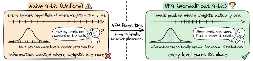
The result: NF4 preserves significantly more of the original model's knowledge than naive 4-bit quantization.

What QLoRA made possible

QLoRA as a technique made it possible to let a person with one high-end GPU do what previously required a multi-node cluster. Thus, the practical barrier to fine-tuning large models dropped by an order of magnitude.

However, there is a tradeoff too. The primary cost of QLoRA is wall-clock time. Every weight that participates in a forward or backward pass must be dequantized on the fly. This extra step adds overhead.

In practice, however, this is almost always an acceptable tradeoff, because the alternative is not "slower training" but rather "no training at all" on a specific piece of hardware.

Quantization beyond training

Quantization is arguably even more impactful at inference time. Serving a model requires fitting it into memory first. Smaller precision means:

• More models per GPU (or larger models on the same GPU)
• Higher throughput (more tokens per second)
• Lower cost per query

Nowadays, it is common practice to deploy LLMs in 8-bit or 4-bit precision. The quality loss is typically negligible for chat and generation tasks. Some deployment setups use mixed precision: 4-bit for most layers and 8-bit or 16-bit for a few layers that are especially sensitive to quantization error.

In summary, both LoRA and QLoRA are essentially ways to minimize changes to the model while still adapting it. They prevent us from having to update billions of weights, making fine-tuning cheaper, and more accessible, and have proven to achieve performance comparable to full model fine-tuning.

Next, let’s explore alignment fine-tuning, where the focus is shaping how a model behaves so its responses better match human intentions and expectations.

Alignment fine-tuning: RLHF, DPO, and GRPO