KV Caching in LLMs, explained visually

​KV caching is a popular technique to speed up LLM inference.

To get some perspective, look at the inference speed difference from our demo:

• with KV caching → 9 seconds
• without KV caching → 40 seconds (~4.5x slower, and this gap grows as more tokens are produced).

Today, let’s visually understand how KV caching works.

Let's dive in!

To understand KV caching, we must know how LLMs output tokens.

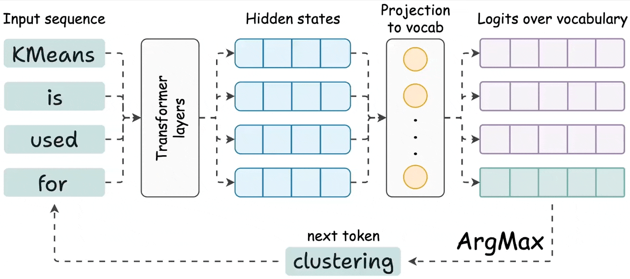
As shown in the visual above:

• Transformer produces hidden states for all tokens.
• Hidden states are projected to vocab space.
• Logits of the last token is used to generate the next token.
• Repeat for subsequent tokens.

Thus, to generate a new token, we only need the hidden state of the most recent token. None of the other hidden states are required.

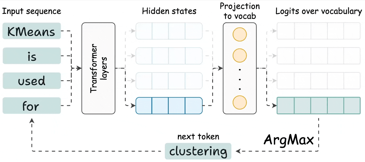
Next, let's see how the last hidden state is computed within the transformer layer from the attention mechanism.

During attention, we first do the product of query and key matrices, and the last row involves the last token’s query vector and all key vectors:

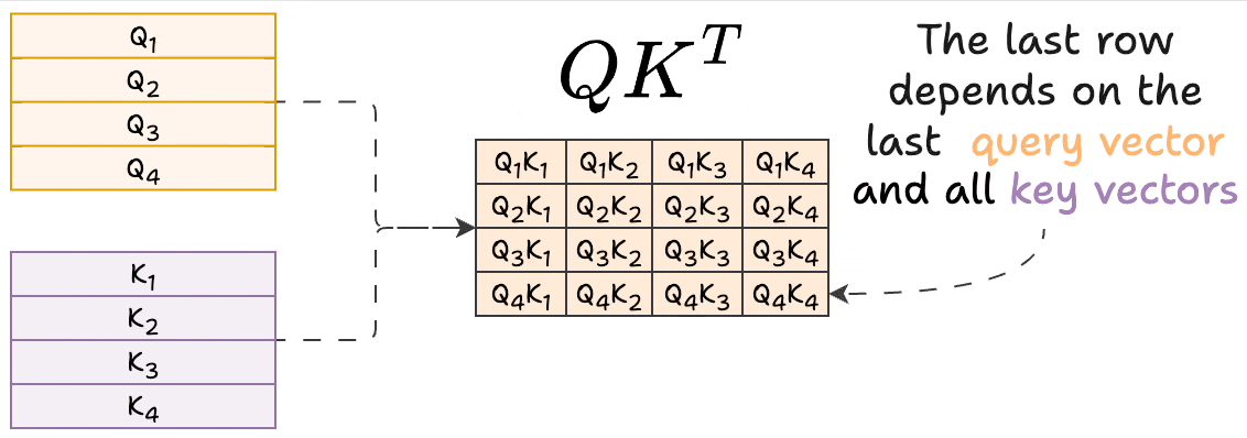
None of the other query vectors are needed during inference.

Also, the last row of the final attention result involves the last query vector and all key & value vectors. Check this visual to understand better:

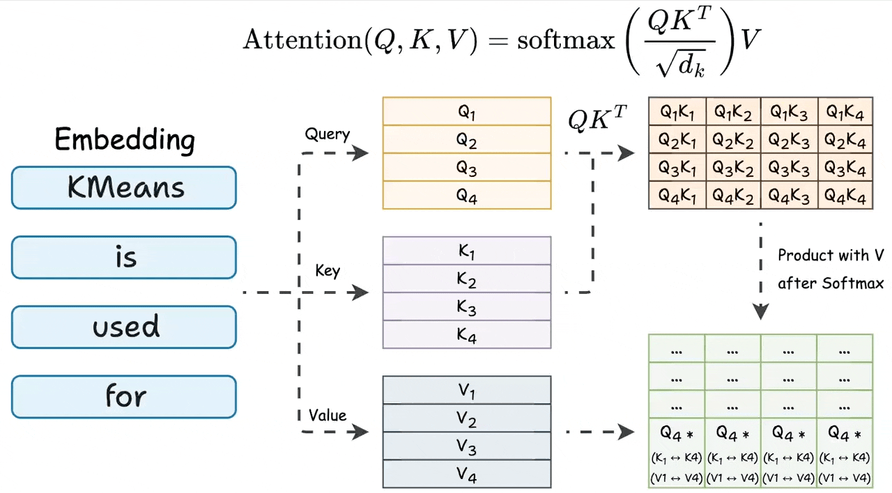
The above insight suggests that to generate a new token, every attention operation in the network only needs:

• Query vector of the last token.
• All key & value vectors.

But there's one more key insight here.

As we generate new tokens, the KV vectors used for ALL previous tokens do not change.

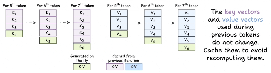
Thus, we just need to generate a KV vector for the token generated one step before.

The rest of the KV vectors can be retrieved from a cache to save compute and time.

This is called KV caching!

To reiterate, instead of redundantly computing KV vectors of all context tokens, cache them.

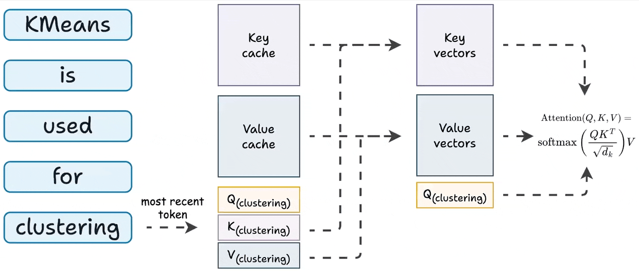
To generate a token:

• Generate QKV vector for the token generated one step before.
• Get all other KV vectors from the cache.
• Compute attention.
• Store the newly generated KV values in the cache.

As you can tell, this saves time during inference.

In fact, this is why ChatGPT takes some time to generate the first token than the subsequent tokens. During that little pause, the KV cache of the prompt is computed.

That said, KV cache also takes a lot of memory.

Consider Llama3-70B, which has:

• total layers = 80
• hidden size = 8k
• max output size = 4k

Here:

• Every token takes up ~2.5 MB in the KV cache.
• 4k tokens will take up 10.5 GB.

More users → more memory.

We'll cover KV optimization soon.

👉 Over to you: How can we optimize the memory consumption?

Thanks for reading!