Understanding LoRA-derived Techniques for Optimal LLM Fine-tuning

👉

Recap

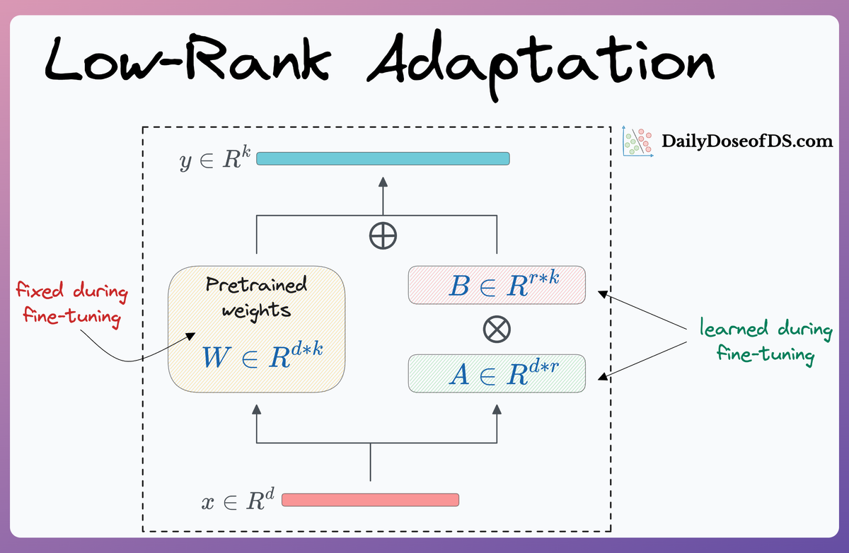
In a recent article, we learned about LoRA, which stands for Low-Rank Adaptation.

It is a technique used to fine-tune large language models (LLMs) on new data. We also implemented it using PyTorch and the Huggingface PEFT library:

As also discussed in the article on vector databases, fine-tuning means adjusting the weights of a pre-trained model on a new dataset for better performance. This is depicted in the animation below:

The motivation for traditional fine-tuning is pretty simple.

When the model was developed, it was trained on a specific dataset that might not perfectly match the characteristics of the data a practitioner may want to use it on.

The original dataset might have had slightly different distributions, patterns, or levels of noise compared to the new dataset.

Fine-tuning allows the model to adapt to these differences, learning from the new data and adjusting its parameters to improve its performance on the specific task at hand.

However, a problem arises when we use the traditional fine-tuning technique on much larger models — LLMs, for instance.

This is because these models are huge — billions or even trillions of parameters, and hundreds of GBs in size.

Traditional fine-tuning is just not practically feasible here. In fact, not everyone can afford to do fine-tuning at such a scale due to a lack of massive infrastructure and the costs associated with such an endeavor.

We covered this in much more detail in the LoRA/QLoRA article, so I would recommend reading that:

Introduction

LoRA has been among the most significant contributions to AI in recent years. As we discussed earlier, it completely redefined our approach to large model fine-tuning by modifying only a small subset of model parameters.

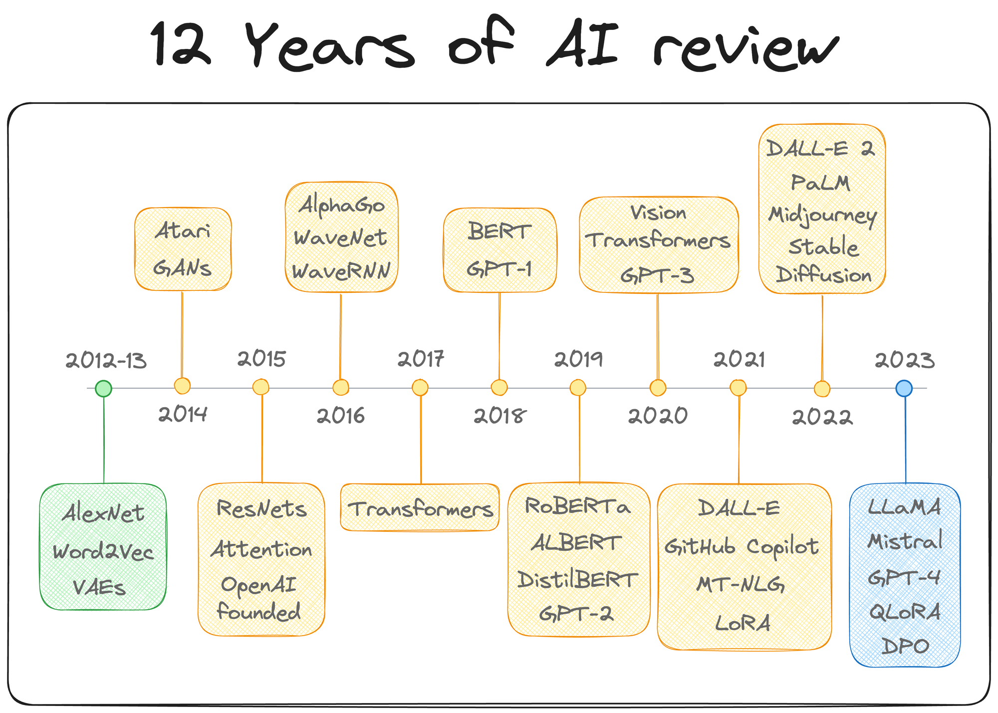
We also mentioned it in the 12 years of AI review we did recently (see year 2021).

Now, of course, it's been some time since LoRA was first introduced. Since then, many variants of LoRA have been proposed, each tailored to address specific challenges and improve upon the foundational technique.

The timeline of some of the most popular techniques introduced after LoRA is depicted below:

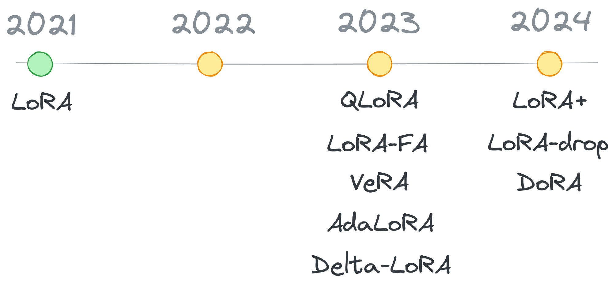
Going ahead, in this article, we will explore the LoRA family in-depth, discussing each variant's design philosophy, technical innovations, and the specific use cases they aim to address.

Let’s begin!

#1) LoRA

The core idea in LoRA, as also discussed in the earlier article, revolves around training very few parameters in comparison to the base model, say, full GPT-3, while preserving the performance that we would otherwise get with full-model fine-tuning (which we discussed above).

More specifically, two low-rank matrices $A$ and $B$ are added alongside specific layers, and these low-rank matrices contain the trainable parameters:

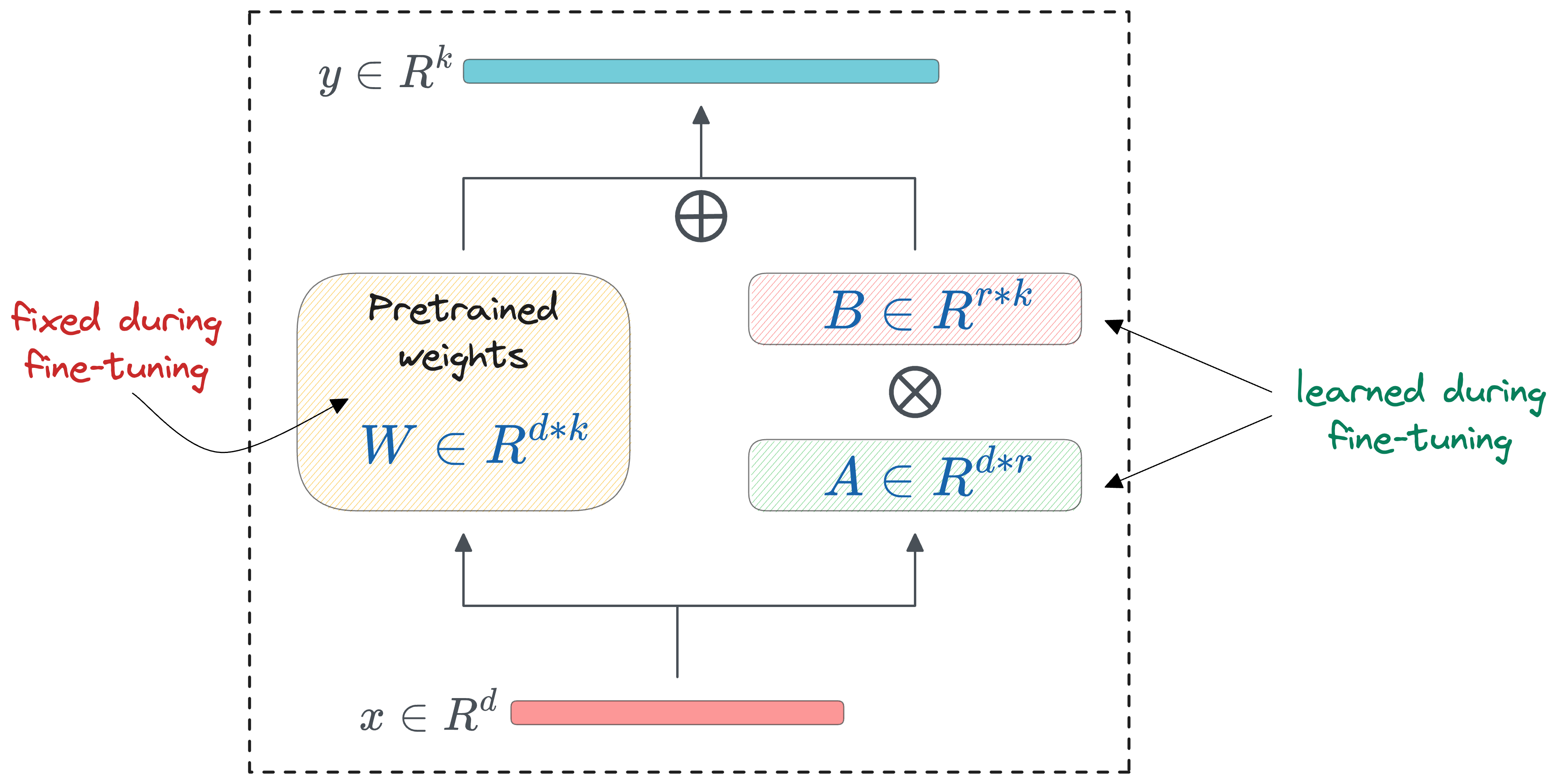
Mathematically, the adaptation is executed by modifying the weight matrix $\Delta W$ in a transformer layer using the formula:

Here, $W$ represents the adapted weight matrix, and $AB$ is the low-rank modification applied to $W$.

As depicted in the LoRA diagram above, the dimensions of matrices $A$ and $B$ are much smaller in size compared to $W$, leading to a significant reduction in the number of trainable parameters.

This low-rank update, despite its simplicity, proves to be remarkably effective in retaining the nuanced capabilities of the LLM while introducing the desired adaptations specific to a new task or dataset.

This way, if there are plenty of users who wish to fine-tune an LLM model (say, from OpenAI), OpenAI must only store the above two matrices $A$ and $B$ (for all layers where this was introduced), which is pretty small in size.

However, the original weight matrix $W$ being common across all fine-tuned versions can have a central version, i.e., one that can be shared across all users.

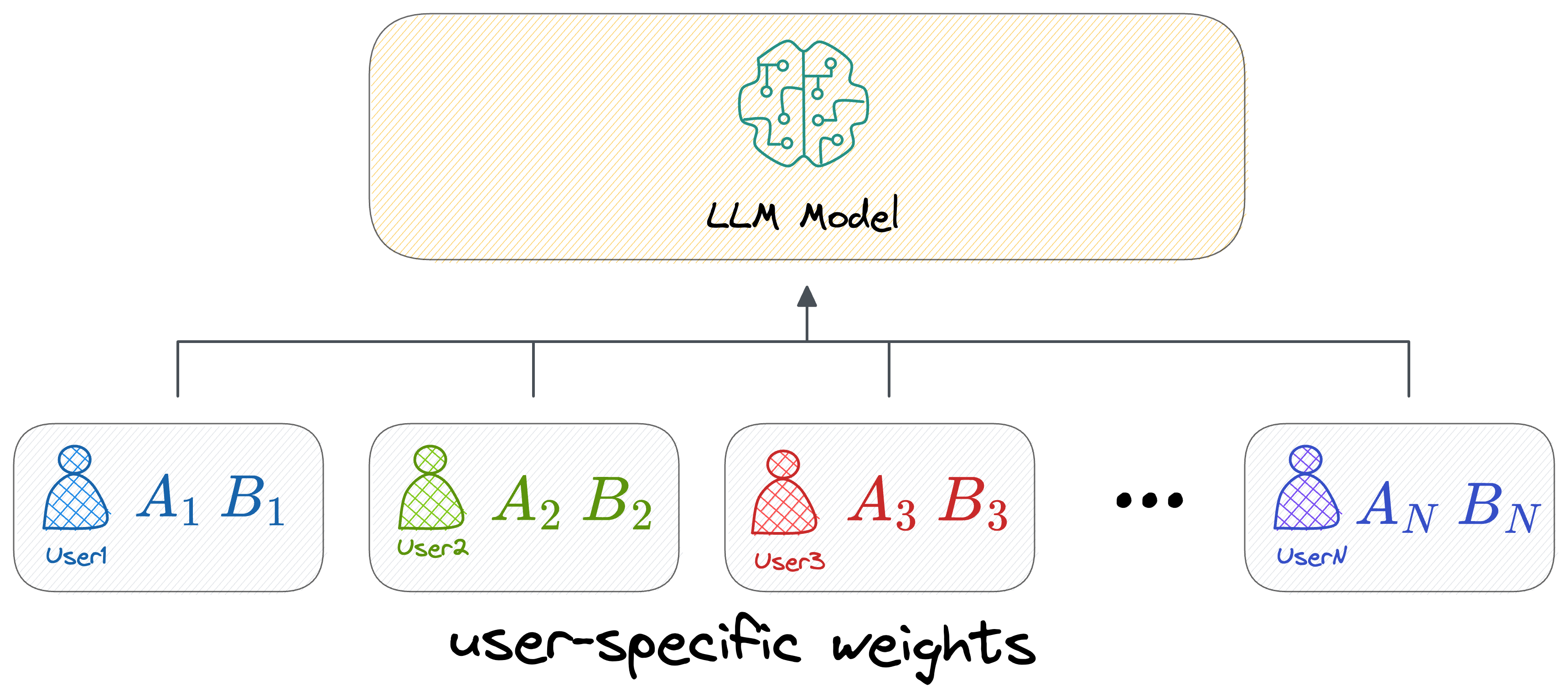
As per the original paper on LoRA, they reduced the checkpoint size by roughly 10,000 times — from 350GB to just 35MB.

Moreover, they also observed a 25% speedup during training on the GPT-3 175B model compared to full fine-tuning, which is pretty obvious because we do not compute the gradient for the vast majority of the parameters.

Another key benefit is that it also introduces no inference latency. This is because of its simple linear design, which allows us to merge the trainable matrices ($A$ and $B$) with the frozen weights ($W$) when deployed, so one can proceed with an inference literally the same way as they would otherwise do.

A pretty cool thing about LoRA is that the hyperparameter $r$ can be orders of magnitude smaller than the dimensions of the corresponding weight matrix.

For instance, in the results table, compare the results of $r=1$ with that of other ranks:

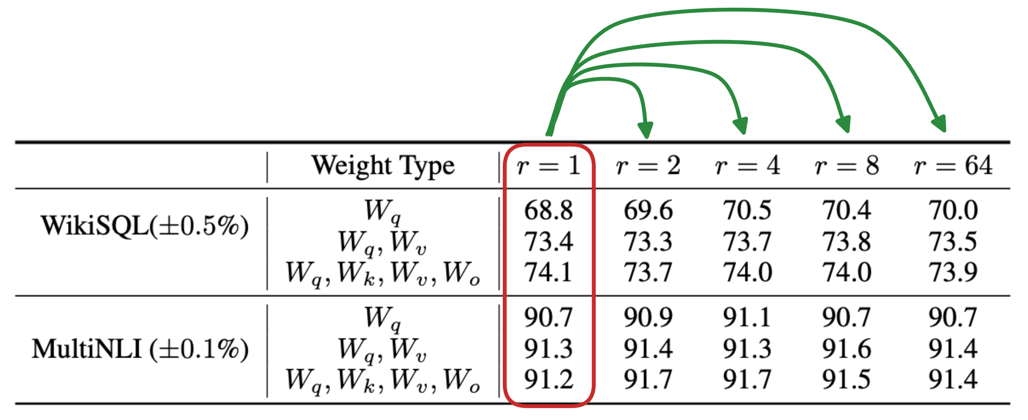
In most cases, we notice that $r=1$ almost performs as well as any other higher rank, which is great!

In other words, this means that the $A$ and $B$ can be a simple row and column matrix.

Next, let’s understand the variants of LoRA and how they differ from LoRA.

#2) LoRA-FA

Introduction

Building on the foundational Low-Rank Adaptation (LoRA) technique, the LoRA-FA method introduces a slight change that reduces the memory overhead associated with fine-tuning large language models (LLMs).