Policy Gradients: REINFORCE and Actor-Critic
Part 7: Learning the policy directly, from REINFORCE to actor-critic.
Recap
In chapter 6, we moved from linear value function approximation to neural networks.
The value function generalized from a linear form to a neural network. What we gave up in that move was the convergence guarantee that held for linear on-policy methods.
We then saw what breaks when deep networks meet online Q-learning: correlated samples, moving targets, and the deadly triad scaled up. Two engineering fixes carried the day:
- Experience replay stored past transitions and sampled them in random minibatches, breaking correlation.

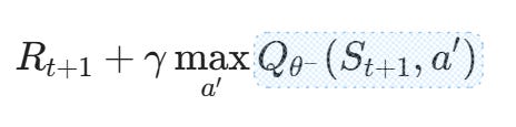
- Target networks froze a copy of the Q-network to compute stable bootstrap targets.
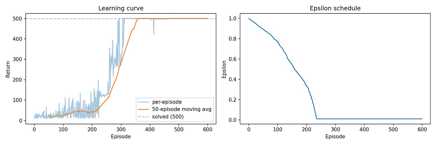
Putting these together gave us DQN algorithm, which we trained from scratch on CartPole.
If you have not read Chapter 6, we recommend doing so first:
Now most of the methods we learned so far share one trait. They learn how good actions are, then derive behavior by picking the best-scoring action. That works beautifully when actions are few and discrete. It strains badly when actions are continuous or numerous.
Hence, there is another way. Instead of scoring actions and choosing among them, we can learn the choosing itself. That is the subject of this chapter.
As for this part, we will focus on policy gradient methods. We will build the policy gradient from first principles, meet REINFORCE, confront its variance problem head-on, and learn about the actor-critic architecture.
Let's begin!
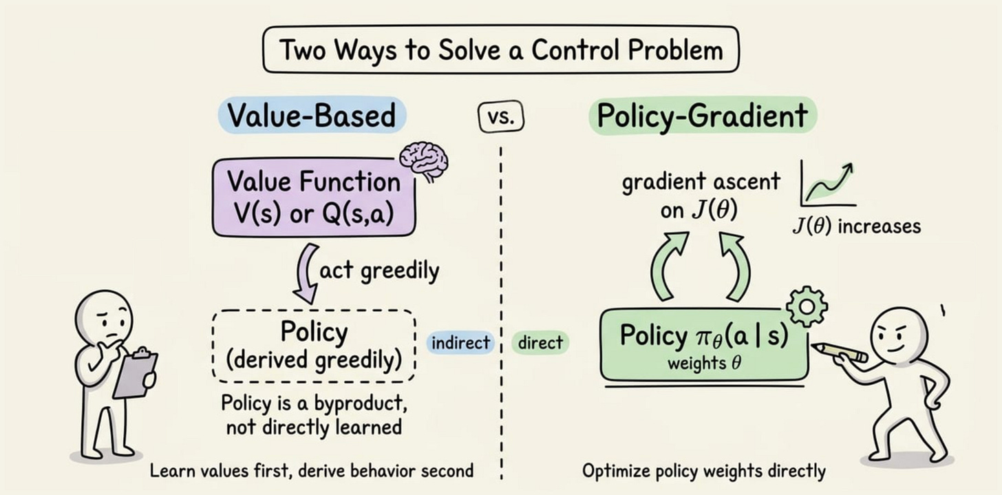
Two ways to solve a control problem
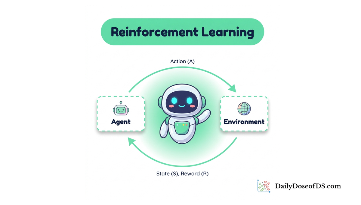
A reinforcement learning agent needs a policy: a rule that says what to do in each state. Up to now, we built that rule indirectly. We learned a value function, an estimate of how much reward we can expect, and then acted greedily with respect to it. The policy was a byproduct of the values.
Policy gradient methods flip this around. They parameterize the policy directly and learn its parameters. We write the policy as a function with its own weights, and we adjust those weights to get better behavior.
Let us make this concrete. A policy maps a state to a distribution over actions. We denote it as follows:
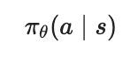
Here $\pi$ is the policy, $\theta$ are its learnable parameters (the weights of a neural network), $s$ is the current state, and $a$ is an action.
This is a stochastic policy and for continuous actions, the network typically outputs the mean and spread of a Gaussian distribution, and we sample from it.
To learn the policy directly, we need an objective: a single number measuring how good the policy is, which we can then push upward. The natural choice is the expected return:
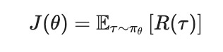
In this expression:
- $J(\theta)$ is the objective we want to maximize, written as a function of the policy parameters $\theta$.
- The symbol $\tau$ (tau) denotes a trajectory, the full sequence of states and actions in an episode.
- The notation $\tau \sim \pi_\theta$ means the trajectory is generated by following the current policy.
- The term $R(\tau)$ is the total return collected along that trajectory.
- $\mathbb{E}[\cdot]$ is the expectation, the average over all the trajectories the policy could produce.
The intuition is direct. If we can compute the gradient of $J$ with respect to $\theta$, we can climb it.
In summary, policy gradient methods learn a parameterized policy by maximizing expected return through gradient ascent. The challenge, which the next section solves, is computing that gradient at all.
The log-derivative trick and the policy gradient theorem
We want the gradient of $J(\theta)$, but there is an immediate obstacle. The objective is an expectation over trajectories, and the distribution of those trajectories itself depends on $\theta$.
Changing the parameters changes which trajectories we see. We cannot simply differentiate inside the average, because the thing we are averaging over is moving as we differentiate.
This is where one elegant identity rescues us. It is called the log-derivative trick, and it rests on a basic fact from calculus. The derivative of the natural logarithm of a function is the derivative of the function divided by the function itself:
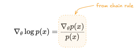
Rearranging it gives the form we actually use: $\nabla_\theta p(x) = p(x) \nabla_\theta \log p(x)$.
Why does this matter? It converts a gradient of a probability into the probability times a gradient of a log-probability. The first form is hard to average over by sampling. The second form is exactly an expectation, which we can estimate by sampling. That single conversion is what makes the whole method work.