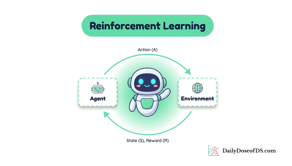
Model-Free Learning

Recap

In the previous chapter, we explored the recursive structure that sits at the heart of reinforcement learning: the Bellman equations.

We started with the Bellman expectation equations for $v_\pi$ and $q_\pi$. We saw that the value of a state, under a fixed policy, equals the expected immediate reward plus the discounted value of the next state. The equations gave us a way to characterize $v_\pi$ and $q_\pi$ exactly, without simulation.

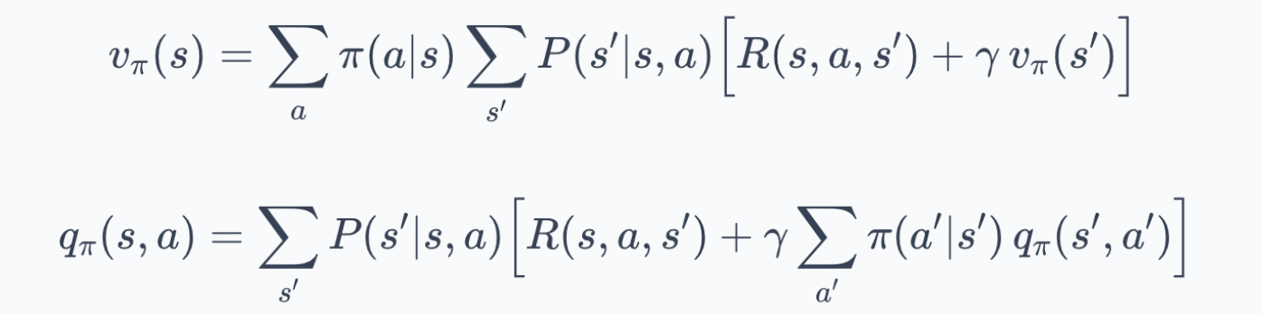
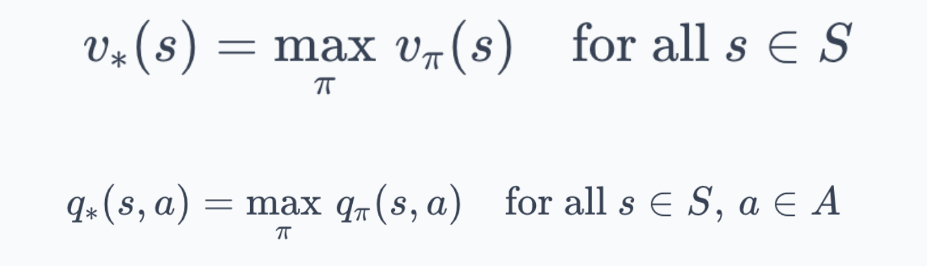
We then derived the Bellman optimality equations for $v_\ast$ and $q_\ast$. These replaced the policy-weighted average with a $max$ over actions, characterizing the best achievable performance in the environment.

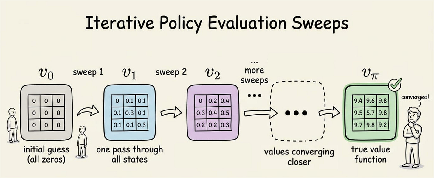
We then turned these equations into algorithms via dynamic programming (DP): policy evaluation, policy improvement, policy iteration, and value iteration.

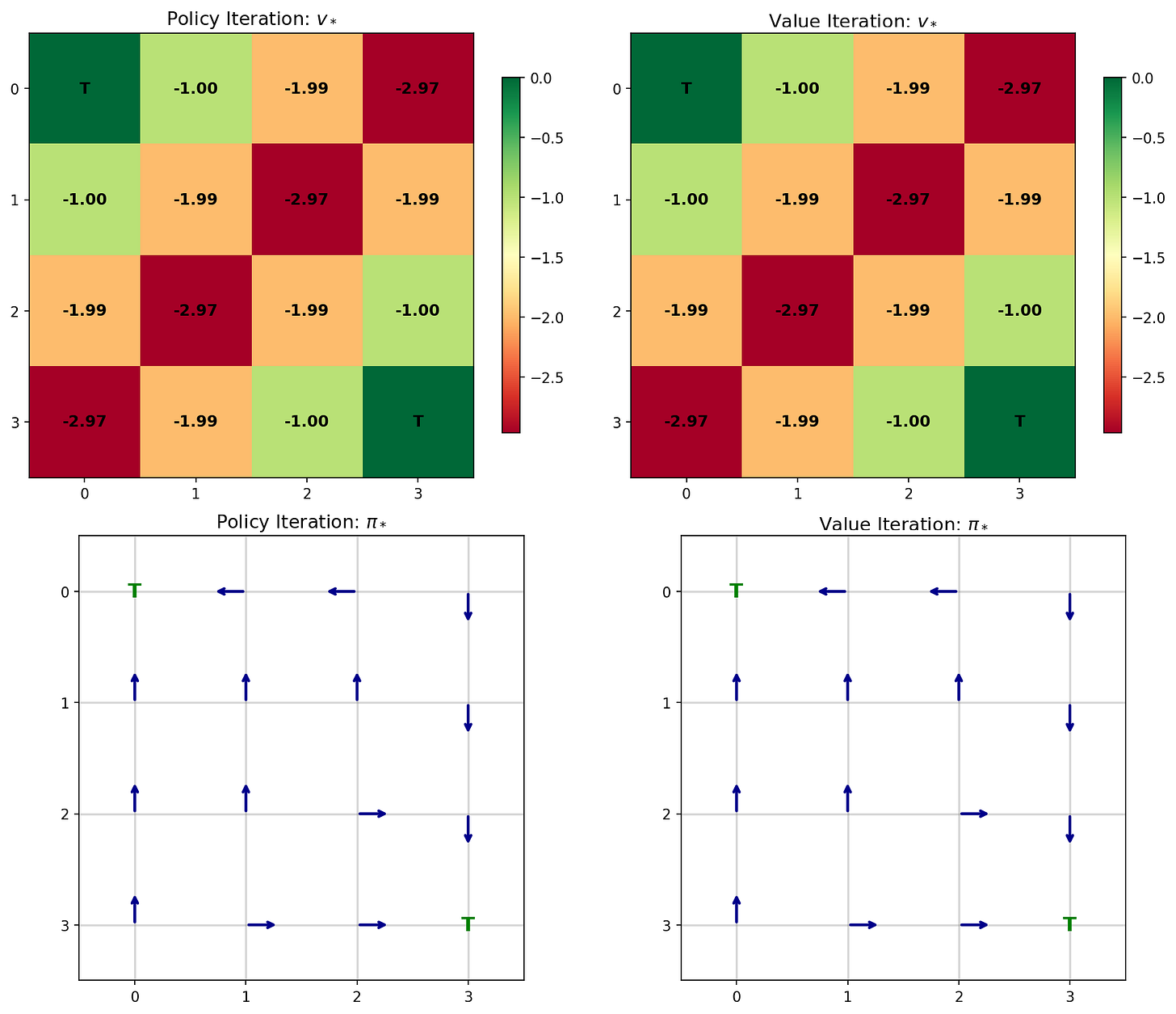
Finally, we ran both policy iteration and value iteration on a 4×4 gridworld and confirmed they converged to the same optimal policy.

If you have not read Chapter 3, we recommend doing so first:

Bellman Equations and Dynamic Programming

RL Part 3: Bellman expectation and optimality equations, policy iteration, value iteration, and why dynamic programming needs a model.

Daily Dose of Data ScienceAvi Chawla

Introduction

DP gave us the gold standard for small, fully known MDPs. The catch is that real environments rarely hand us a clean $P$ and $R$.

What we usually do have is something else: an agent that can interact with the environment, take actions, and observe rewards and next states. The question for this chapter is how to estimate value functions and learn good policies purely from this kind of experience, without any access to $P$ or $R$.

This is the model-free setting.

We will look at two foundational families:

• Monte Carlo (MC) methods, which learn from full episodes of experience.
• Temporal-difference (TD) methods, which learn from single transitions by using their current estimates to update themselves.

From there, we will move to TD-based control: SARSA and Q-learning, and close with an experiment that contrasts the two.

Let's begin!

What model-free actually means?

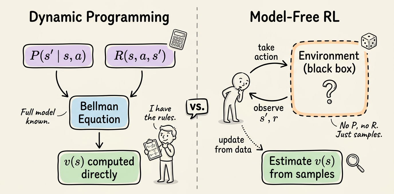
Although we briefly introduced the idea of model-free learning in Chapter 2, it is worth revisiting now. A helpful way to contextualize the term is by contrasting it with the methods explored in Chapter 3.

In DP, we plugged $P$ and $R$ directly into the Bellman update. The agent never had to do anything. We computed $v_\pi$ or $v_*$ by sweeping over the state space and applying the equations. There was no interaction with the environment, no episodes to play out and no exploration to manage. We treated the environment as a known mathematical object.

In model-free RL, we do not have $P$ or $R$. We have an agent that can be placed in a state, take an action, and observe the resulting next state and reward. From these samples, we estimate value functions and improve policies. The environment is treated as a black box.

Two organizing axes will run through the rest of the chapter:

• The first is prediction versus control. Prediction is the task of estimating $v_\pi$ or $q_\pi$ for a given fixed policy. Control is the task of finding a good policy.

• The second axis is on-policy versus off-policy. An on-policy method learns about the same policy it uses to generate behavior. An off-policy method can learn about one policy (the target policy) while behaving according to another (the behavior policy).

So now, let's dive into understanding the various model-free techniques.

Monte Carlo prediction

We know that the value of a state under a policy is, by definition, the expected return when starting from that state and following the policy: