Markov Decision Processes and Value Functions

Recap

In the previous chapter, we introduced reinforcement learning as a third kind of machine learning, distinct from supervised and unsupervised learning.

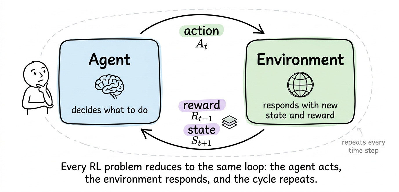
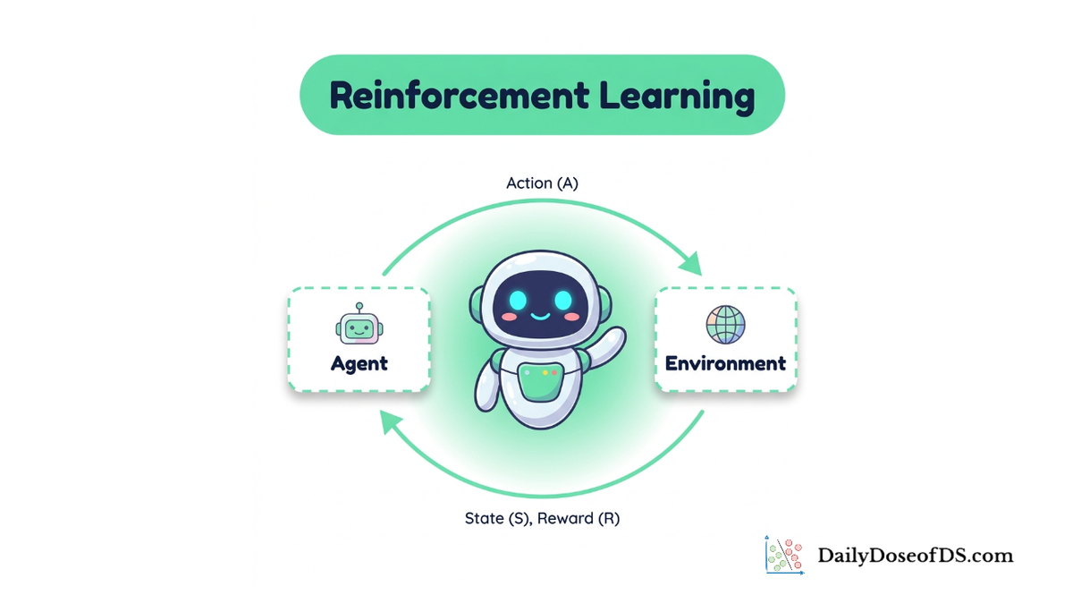
We saw the core agent-environment loop, where the agent picks actions, the environment returns rewards and a new state, and the cycle continues.

We discussed four properties that make RL distinctive: feedback is evaluative rather than instructive, the data distribution depends on the agent's own behavior, consequences are delayed and create the credit assignment problem, and exploration cannot be avoided.

We then studied the simplest possible RL problem: the multi-armed bandit. With no states to track, only $k$ actions and unknown reward distributions, the bandit isolates the exploration-exploitation tradeoff.

We worked through four strategies, namely greedy, $ε$-greedy, optimistic initial values, and upper confidence bound (UCB), and ran them on the 10-armed testbed to see how each one trades off exploration against exploitation in practice.

Overall, the previous chapter familiarized us with some of the most basic ideas of reinforcement learning.

If you haven’t yet gone through Part 1, we recommend reviewing it first, as it establishes the conceptual foundation essential for understanding the material we’re about to cover.

Read it here:

Foundations of Reinforcement Learning

RL Part 1: Agents, environments, rewards, and why RL is different from supervised learning.

Daily Dose of Data ScienceAkshay Pachaar

In this chapter, we will understand and explore the Markov property, Markov decision processes (MDPs), value functions and much more.

As always, every notion will be explained through clear examples and walkthroughs to develop a solid understanding.

Let's begin!

Introduction

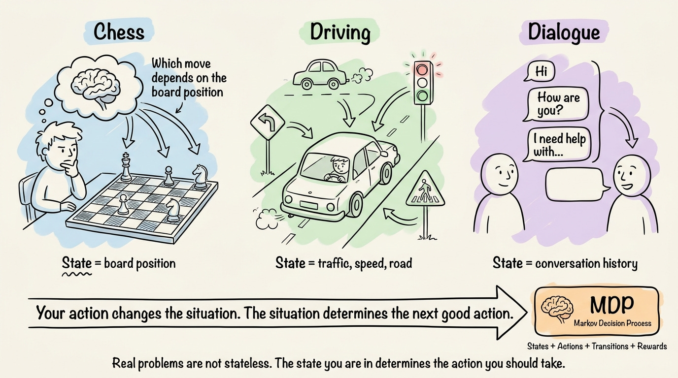
In Chapter 1, the bandit gave us a clean way to think about exploration and exploitation. But it hid a detail that changes a lot of things. Real problems are not stateless.

In chess, the move you should make depends on the current board position. In driving, the next steering action depends on the surrounding traffic. In a dialogue, what to say next depends on the conversation so far. The action you take changes the situation you face afterward, and the situation determines which actions are good.

To talk about states, transitions, and how rewards depend on both, we need a formal vocabulary.

That vocabulary is the Markov decision process (MDP), and it underpins essentially every algorithm we will study.

We will explore the framework of MDPs. We will start with the Markov property, which is what makes the whole edifice tractable. We will then formalize the MDP itself and discuss episodic versus continuing tasks. From there, we will define the return, discounting, and the reward hypothesis.

We will introduce policies as the object the agent actually learns, and define two value functions, $v_π$ and $q_π$​, that measure how good states and actions are under a given policy.

Finally, we will build a small gridworld from scratch and use Monte Carlo rollouts to estimate $v_π$​ for a fixed policy.

The Markov property

Before defining what an MDP is, we need the assumption it rests on: the Markov property.

Informally, a state is Markov if the future depends on the past only through the present. This means that once you know the current state, the entire history that led to it is irrelevant for predicting what happens next.

Formally, the state $S_t$​ is Markov if the distribution of the next state conditioned on the entire history reduces to a distribution conditioned only on the current state and action:

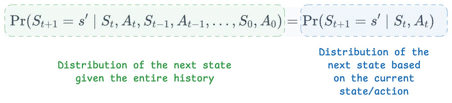
Here, $S_{t+1}$​ is the resulting next state, and $s′$ is a particular value the next state can take. The left side is the probability of landing in $s′$ given the entire history of states and actions. The right side is the same probability, but conditioned only on the current state and action.

The Markov property says these two are equal.

This has enormous benefits.

Without it, predicting the next state would, in principle, require remembering everything the agent has ever seen. With it, we only need the current state. The state is a complete summary of the past, sufficient to predict the future.

Here's a concrete example. Consider the Atari game Breakout, with the bat at the bottom and a ball bouncing around.

If we treat a single screenshot as the state, is the state Markov? The answer is no.

From one frame, you cannot tell which direction the ball is moving. There are at least four directions consistent with any given frame, and they lead to very different next states.

But what if the state is the past four frames stacked together? Now you can compute the ball's position and velocity, and the next frame becomes predictable. The state, redefined this way, is approximately Markov.

This points to something important. "Markovian-ness" is often a modeling choice, not a physical fact. The same physical environment can be Markov or not, depending on what you decide to put in the state.

When the property genuinely cannot hold, the agent only sees observations that are partial summaries of a true underlying state it cannot directly access.

This setting has its own name, which is called the partially observable Markov decision process (POMDP), introduced by Karl Johan Åström in 1965 for the discrete state space.

In a POMDP, the true state can be called hidden, not in the sense of being deliberately concealed, but in the sense that the agent only sees it indirectly through observations. POMDPs add an observation set and an observation function, and require the agent to track a probability distribution over what the hidden state might be, called a belief.

At this point, we must also understand that the Markov property does not say states are deterministic. The next state is allowed to be random. The property only says the randomness depends solely on the current state and action.

With the Markov property in place, we can now formalize the agent-environment interaction as a tuple of components, each playing a specific role.

The MDP framework

A Markov decision process is a 5-tuple: