Bellman Equations and Dynamic Programming

Recap

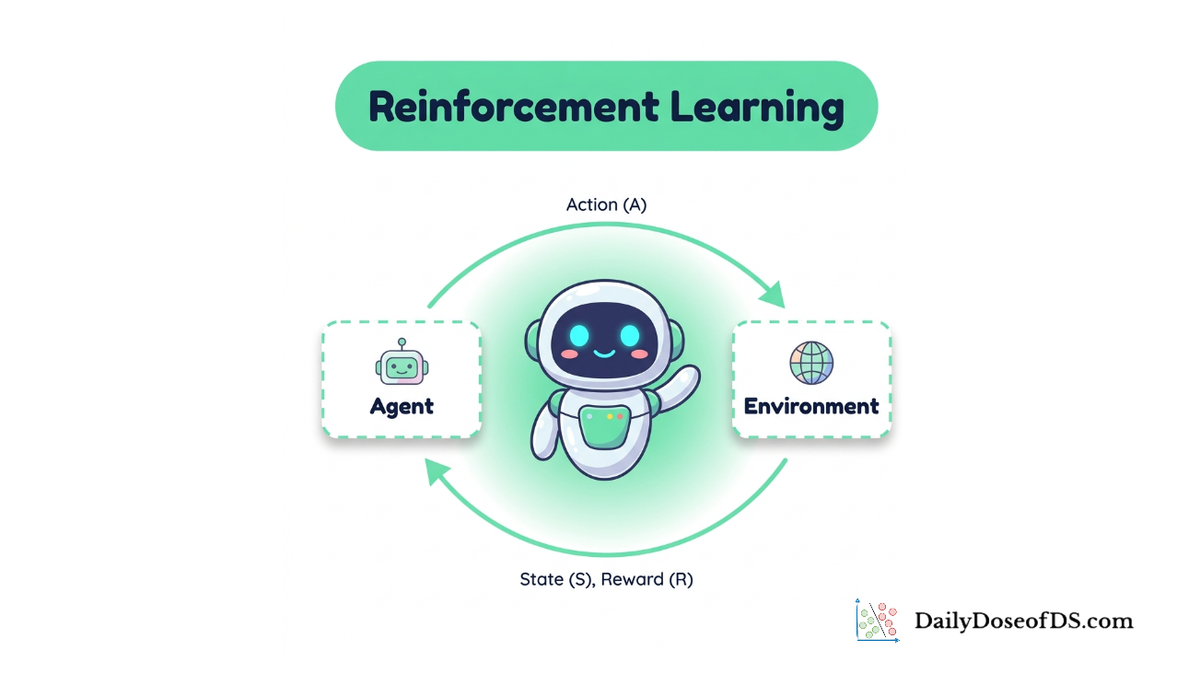
In the previous chapter, we formalized the agent-environment interaction as a Markov decision process (MDP).

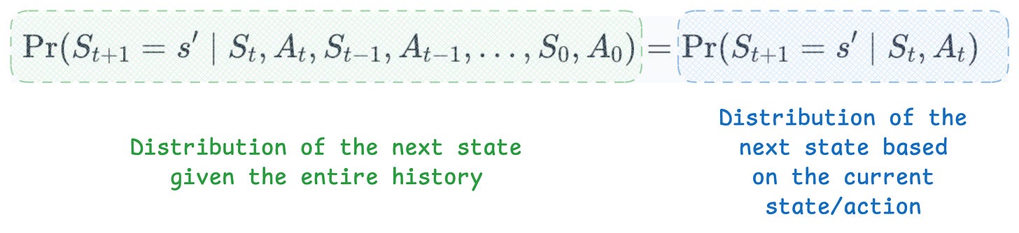
We began with the Markov property, which states that the future depends on the past only through the present state. This is the assumption that makes the entire framework tractable: once you know the current state, you can discard the history.

We then defined the MDP as a 5-tuple $(S, A, P, R, \gamma)$: states, actions, a transition function, a reward function, and a discount factor.

We discussed episodic versus continuing tasks. We defined the return $G_t$ as the discounted cumulative reward, and explained how $\gamma$ controls the agent's far-sightedness.

We introduced policies, both deterministic and stochastic, as the object the agent learns. We defined the state-value function $v_\pi(s)$ as the expected return from state $s$ under policy $\pi$, and the action-value function $q_\pi(s,a)$ as the expected return from taking action $a$ in state $s$ and then following $\pi$.

Finally, we built a 4×4 gridworld and used Monte Carlo rollouts to estimate $v_\pi$ for a random policy.

If you have not read Chapter 2, we recommend doing so first:

Markov Decision Processes and Value Functions

RL Part 2: Markov decision processes, returns, policies, and value functions.

Daily Dose of Data ScienceAvi Chawla

Introduction

In Chapter 2, we computed $v_\pi$ by running thousands of episodes and averaging the returns.

Recall that $v_\pi(s)$ tells us how much total reward the agent can expect to collect starting from state $s$ if it follows policy $\pi$.

In Part 2, we estimated this the brute-force way. Drop the agent into a state, let it act until the episode ends, write down the total reward, and do that thousands of times. Average those numbers and you get $v_\pi(s)$.

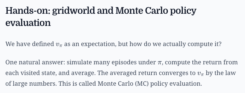
The approach works, but it is expensive and noisy. Each estimate is a sample average, and the variance shrinks slowly.

There is a more direct route. The value functions satisfy recursive equations that relate the value of a state to the values of its successor states. These are the Bellman equations, named after Richard Bellman, who introduced the principle of optimality and the method of dynamic programming and compiled them into his landmark 1957 book "Dynamic Programming" (Princeton University Press).

The Bellman equations give us two things. First, they characterize $v_\pi$ and $q_\pi$ exactly, without simulation. Second, they characterize the optimal value functions $v_\ast$ and $q_\ast$, which tell us the best possible performance in the environment.

Dynamic programming (DP) turns these equations into algorithms. Given a complete model of the environment (the transition function $P$ and the reward function $R$), DP computes optimal policies exactly and efficiently for small problems.

In this chapter, we will derive the Bellman expectation equations for $v_\pi$ and $q_\pi$, then the Bellman optimality equations for $v_\ast$ and $q_\ast$.

We will also study four DP components: policy evaluation, policy improvement, policy iteration, and value iteration. We will close with a hands-on project, running both policy iteration and value iteration on the 4×4 gridworld and comparing the results side by side.

Let's begin!

The Bellman expectation equation for $v_\pi$

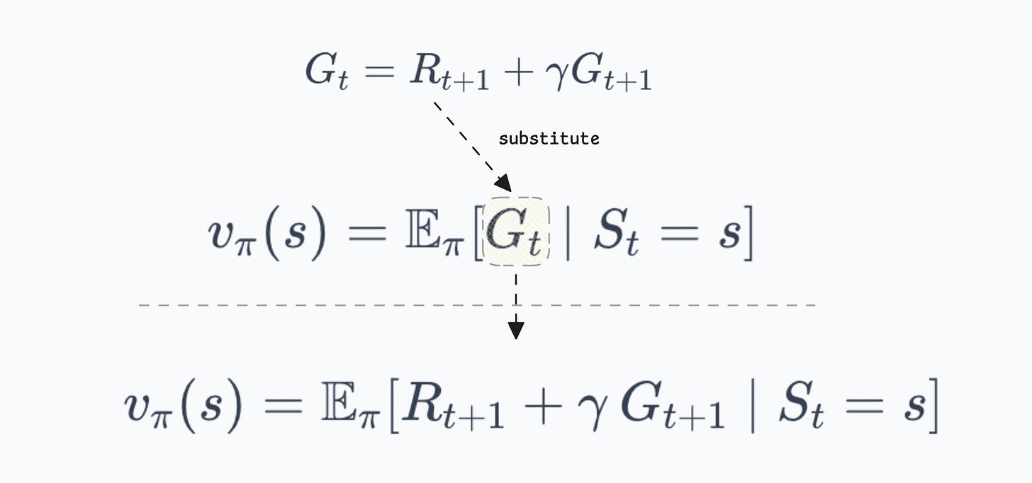
In Chapter 2, we established the recursive structure of the return:

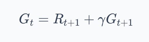
If this looks unfamiliar, $G_t$ is just the return, the total (discounted) reward the agent collects from time step $t$ onward.

We defined it in Part 2 as described above. The recursive version above says that the total reward is whatever you get right now, plus $\gamma$ times everything you get after that.

The state-value function is the expected return from state $s$ under policy $\pi$:

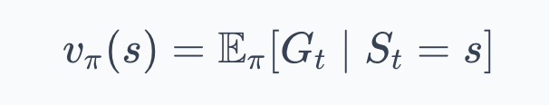
As we covered in Part 2, this expectation accounts for two kinds of randomness:

→ The agent might act randomly (because $\pi$ can be stochastic)

→ The environment might respond randomly (because $P$ can be stochastic).

The value $v_\pi(s)$ averages over both.

Substituting the recursive return into this expectation and expanding gives us the Bellman expectation equation for $v_\pi$. The derivation proceeds in a few steps:

1. Starting from the definition, we substitute the recursive return:

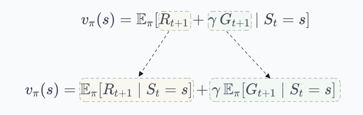
2. Expectation is linear, so we can split it:

3. Now we need to expand these expectations. The agent is in state $s$ and selects action $a$ according to $\pi(a|s)$. The environment then transitions to state $s'$ with probability $P(s'|s,a)$ and emits reward $R(s,a,s')$. Expanding over actions and next states:

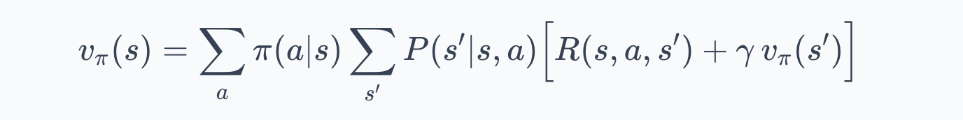
This is the Bellman expectation equation for $v_\pi$.

Let us unpack everything here:

• $v_\pi(s)$ is the value of state $s$ under policy $\pi$.
• The outer sum runs over all actions $a$ available in $s$, each weighted by $\pi(a|s)$, the probability the policy assigns to that action.
• The inner sum runs over all possible next states $s'$, each weighted by $P(s'|s,a)$, the transition probability. Inside the brackets, $R(s,a,s')$ is the immediate reward for the transition, and $\gamma \, v_\pi(s')$ is the discounted value of the successor state.

The structure has two layers. The outer layer averages over the agent's action choice (governed by $\pi$). The inner layer averages over the environment's response (governed by $P$). The term in brackets combines the immediate reward with the future value, discounted by $\gamma$.

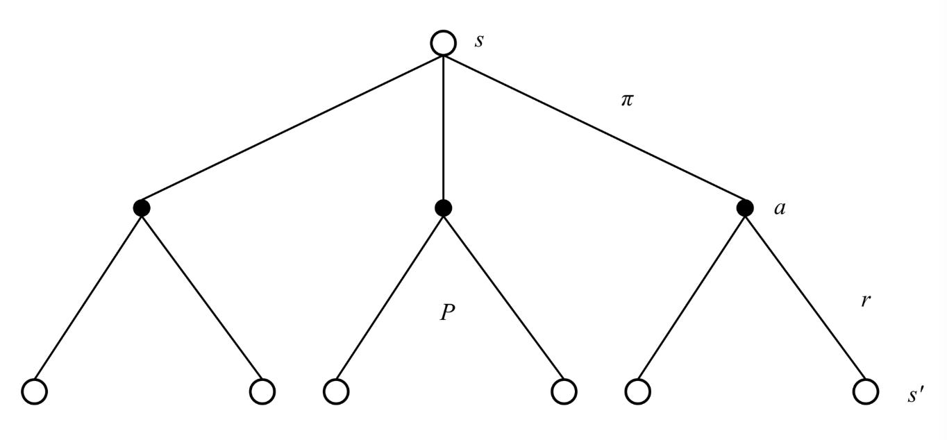
The intuition is that the value of a state equals the average immediate reward plus the average discounted value of wherever you end up next, where "average" accounts for both the policy's randomness and the environment's randomness. If $\gamma = 0$, only the immediate reward matters. If $\gamma = 1$, the future matters as much as the present.

A concrete example

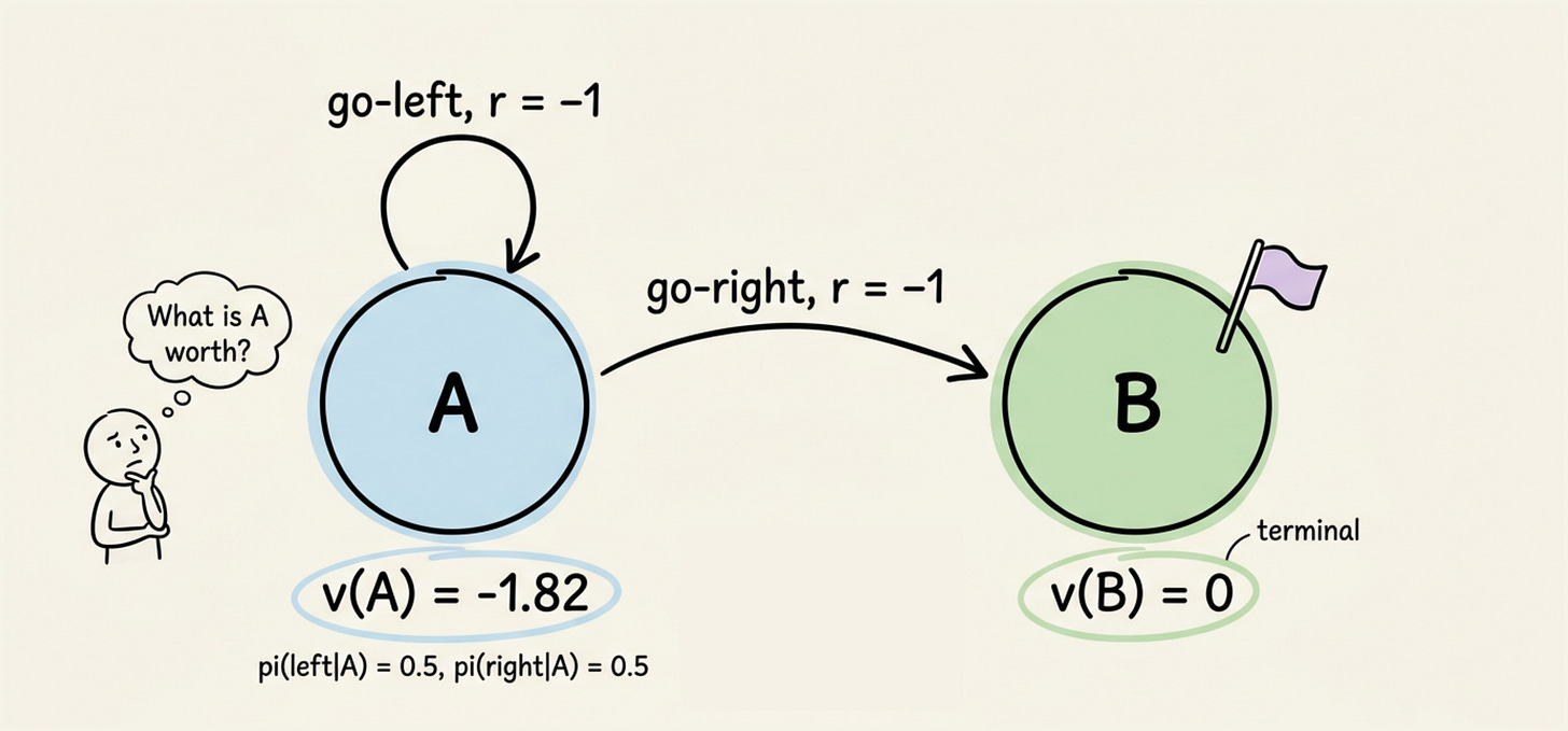
Consider a tiny two-state MDP to see the equation at work:

State A has two actions:

• go-left (stays in A)
• go-right (moves to terminal state B).

The policy $\pi$ is: $\pi(\text{left}|A) = 0.5$, $\pi(\text{right}|A) = 0.5$. Every transition gives a reward $-1$. Transitions are deterministic. The discount factor is $\gamma = 0.9$.

Since B is terminal, $v_\pi(B) = 0$. For state A, the Bellman equation gives:

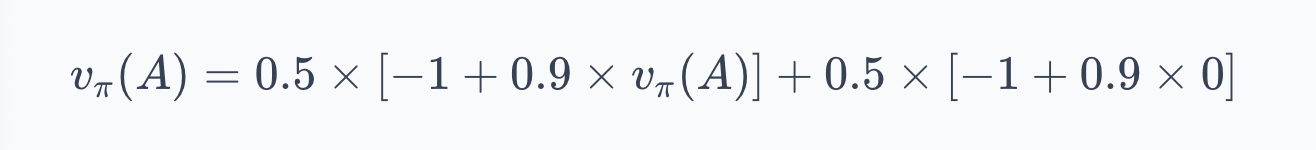
The first term covers go-left: reward $-1$, then back to A. The second covers go-right: reward $-1$, then terminal. Solving:

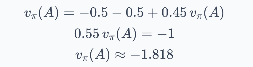
Under this policy, the agent expects about $-1.82$ in total return from state A. The negative value reflects the $-1$ cost per step and the 50% chance of looping. If the policy always went right, the value would be simply $-1$: one step, one reward, done.

Now let's go ahead and understand the Bellman expectation equation for $q_\pi$.

The Bellman expectation equation for $q_\pi$