Introduction to Deep RL and DQN

Recap

In the previous chapter, we made the transition from tables to parameterized value functions.

The reasons were structural. Tables do not scale, and they do not generalize. Mountain car has a state space made of two real numbers, so it is impossible to even index into a table for it. And updating one cell of a Q-table tells us nothing about the cell next to it. The fix was to write the value function as a function over states, with a small parameter vector $\theta$ controlling its shape.

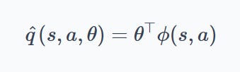
We laid out the prediction objective, mean square value error. We then worked through linear function approximation in detail, where the value estimate is the inner product of fixed features and learnable weights.

From that foundation, we built two learning algorithms:

• Gradient Monte Carlo uses the full return as a target, which makes it a true gradient method on a well-defined squared-error objective.

• Semi-gradient TD(0) replaces the return with a bootstrapped target, gaining online updates and low variance, but introducing the bias of differentiating only the prediction and not the target.

We then extended our understanding to control:

• Semi-gradient SARSA learns the action-value function on-policy and works reliably with linear features.

• Semi-gradient Q-learning uses the max over next actions, making it off-policy. This places it squarely inside what Sutton and Barto call the deadly triad: function approximation, bootstrapping, and off-policy learning combined.

Finally in the hands-on section, we saw the deadly triad cause divergence on Baird's counterexample, a tiny seven-state MDP where the weights grow without bound even though the true value function is zero everywhere.

We also saw the other side of the picture with semi-gradient SARSA on Mountain Car. Tile coding gave us a useful continuous-state representation, and the cost-to-go surface reconstructed the underlying physics of the task.

If you have not read Chapter 5, we recommend doing so first:

Function Approximation

RL Part 5: From tables to parameterized value functions.

Daily Dose of Data ScienceAvi Chawla

Introduction

The deadly triad demonstration at the end of Chapter 5 made one thing clear. Combining function approximation, bootstrapping, and off-policy learning creates a real risk of divergence, and that combination is exactly what we want for scalable value-based RL:

• We want function approximation because tables do not scale.
• We want bootstrapping because waiting for full returns is slow.
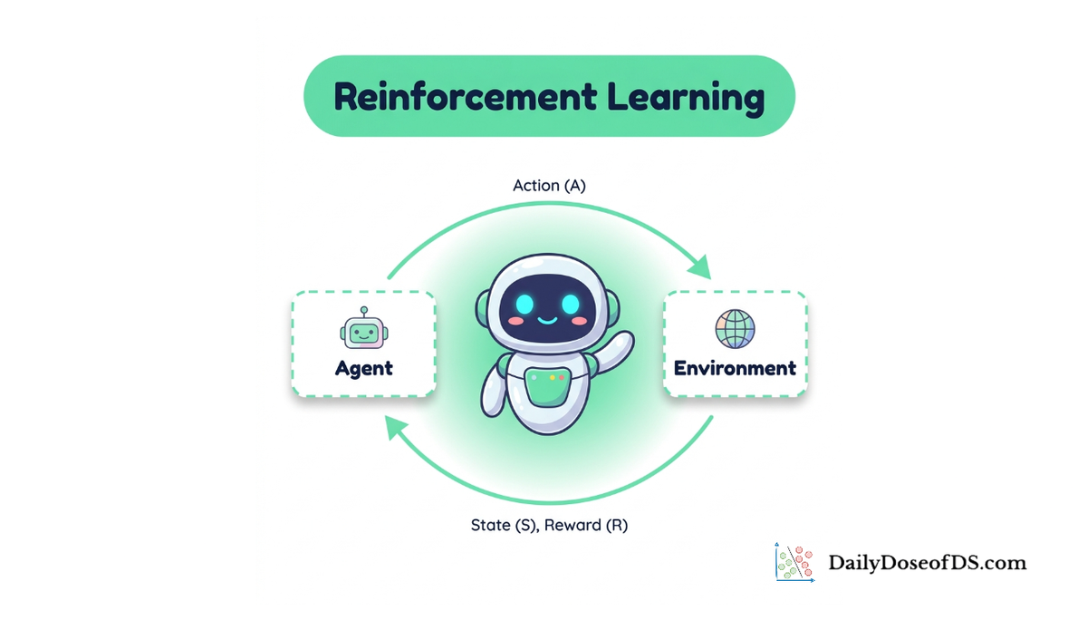
• We want off-policy learning because we want to learn about an optimal greedy policy while exploring with a softer one.

This chapter is about how the field made that combination work in practice.

We will extend the function class from linear to neural, watch new instabilities emerge in the deep setting, and see how DQN's two engineering choices, experience replay and target networks, tame them. The chapter then closes with a hands-on experiment training a DQN agent on CartPole.

Let's begin!

From linear to neural

The mechanical step from linear function approximation to neural function approximation is small. We already know the action-value function as a linear combination of features:

The shift is to replace this expression with a more general parameterized function:

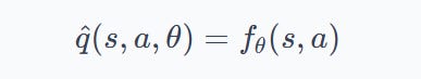
where, $f_\theta$ is now any function differentiable in $\theta$, typically a neural network.

The structure tells us the key change. With linear FA, the features carried the inductive bias and the weights did the learning. With neural FA, the network does both. Nothing about the underlying RL problem changes.

The MDP is the same, the Bellman equations are the same, only the function class used to approximate the value function has grown.

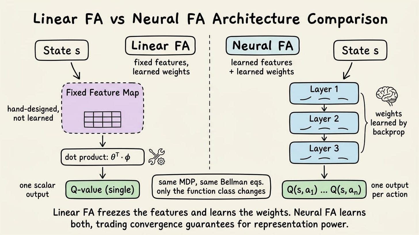
The reason we want this change is representation learning. Hand-designed features work well when the state space is low-dimensional and we know what matters. But for higher dimensions, we almost always have no idea what the right features are. A neural network discovers them from data.

The trade-off is theoretical. In Chapter 5, we noted that linear on-policy semi-gradient TD converges to a unique fixed point. That result depends on linearity. With nonlinear function approximation, even on-policy semi-gradient TD can diverge.

So moving to neural networks gives up the theoretical guarantees we had with linear FA, even before we add off-policy learning back into the mix.

The field accepts this trade-off because the empirical results justify it, and because engineering choices make the situation tractable in practice.

In summary, the move to neural function approximation is a small mechanical change that buys us representation learning, at the cost of the convergence guarantees we had with linear features.

The rest of the chapter is about what goes wrong when we make this move, and what we do about it.

The naive approach and what breaks

Let's try the most direct approach. Take semi-gradient Q-learning from Chapter 5, swap the linear function for a neural network, and run it online.

The update rule is:

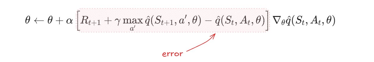
The terms:

• The bracketed expression is the TD error.
• $\nabla_\theta \hat{q}(S_t, A_t, \theta)$ is the gradient of the predicted Q-value with respect to all network parameters, computed by backpropagation.
• $\alpha$ is the step size.

In structure, this is identical to what we had with linear FA. The only difference is what $\hat{q}$ and its gradient look like under the hood.

Run this loop on a problem like CartPole, and the agent learns nothing. Often, the weights drift, the loss climbs, and the agent's behavior gets worse over time.

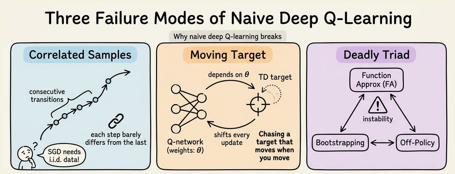
There are three reasons, and each one maps back to something we already discussed in Chapter 5:

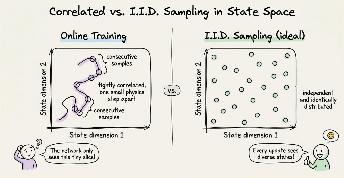
• The first problem is sample correlation. In online learning, the data we train on comes from consecutive transitions in the environment. Two consecutive states in CartPole differ by one small physics step. Thus two consecutive samples are not independent, they are tightly correlated. Stochastic gradient descent assumes (or at least works much better with) approximately independent and identically distributed samples. When samples come in a correlated sequence, the network overfits to whatever local region of the state space the agent happens to be in, and forgets about regions it visited earlier.

• The second problem is non-stationary targets. The TD target $R_{t+1} + \gamma \max_{a'} \hat{q}(S_{t+1}, a', \theta)$ depends on $\theta$. Every time we take a gradient step, the target shifts too. We are trying to fit a moving target, and the moving target depends on us. In Chapter 5 we spelled this out as the core of the semi-gradient idea: we differentiate only the prediction, not the target. With linear FA and on-policy sampling, this was tolerable. But with neural FA and off-policy sampling, the same trick stops being tolerable. A small change in $\theta$ propagates through the network and can change the predicted value at many states at once, including the next state we are about to bootstrap from. The target now moves in unpredictable directions every update.
• The third problem is the deadly triad in full nonlinear form. We are using function approximation (the network), bootstrapping (the TD target), and off-policy learning (the max over next actions). This is exactly the combination Baird's counterexample showed was unstable, and now we are scaling it up to a much larger function class.

This was the situation in 2013, when Mnih et al. published "Playing Atari with Deep Reinforcement Learning". It was the first deep learning model to successfully learn control policies directly from high-dimensional sensory input using reinforcement learning.

The contribution was not the basic idea of combining Q-learning with a neural network. That had been tried before. The contribution was the engineering choices that made it work: experience replay and, in the 2015 Nature version, target networks. We turn to those next.

Experience replay

The first of DQN's two engineering choices is experience replay.