Speculative Decoding in LLMs

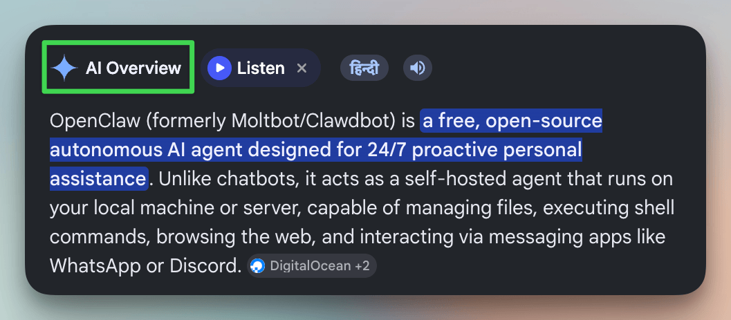
Google uses speculative decoding in AI Overviews to serve over a billion Search users.

It’s also how Anthropic, Meta, and most major inference providers reduce latency at scale and get 2-3x more tokens per second, with mathematically identical outputs.

We covered the mechanics of LLM inference (prefill and decode phases, KV caching, speculative decoding, batching, and optimization techniques that improve latency and throughput here in the LLMOps course →

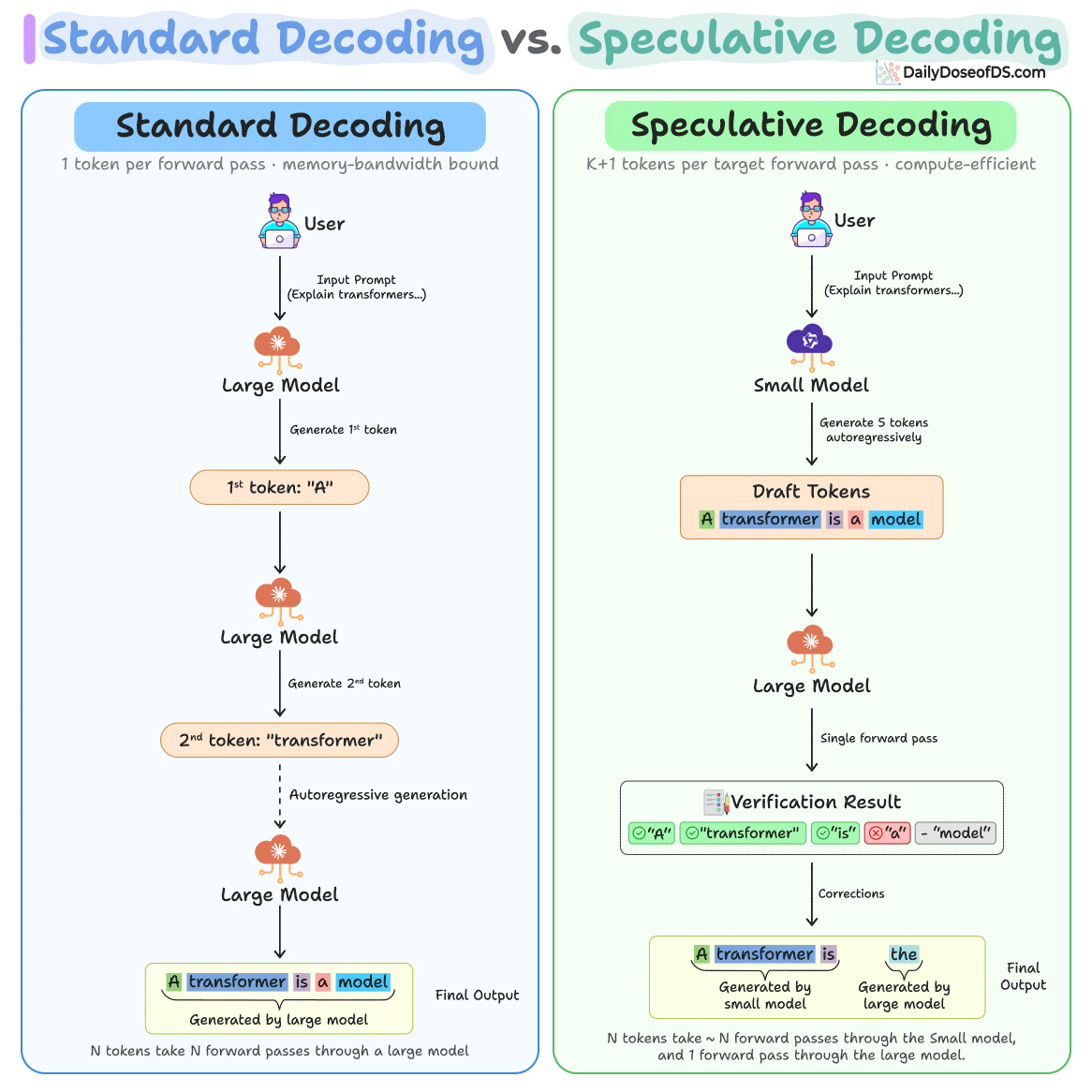
The idea comes from CPU architecture. A small draft model proposes several tokens ahead, and then a large model verifies them all in a single forward pass. Correct predictions (which are typically 60-80% of tokens) get accepted at the inference cost of the small model.

The diagram below depicts how speculative decoding differs from standard decoding:

Let's dive in to understand the key problem it solves and how it works!

The problem

A 70B parameter model in FP16 occupies roughly 140 GB of GPU memory.

During the decode phase, EVERY SINGLE TOKEN requires a full forward pass through all 70B parameters (due to autoregressive generation), reading the entire model weights from memory.

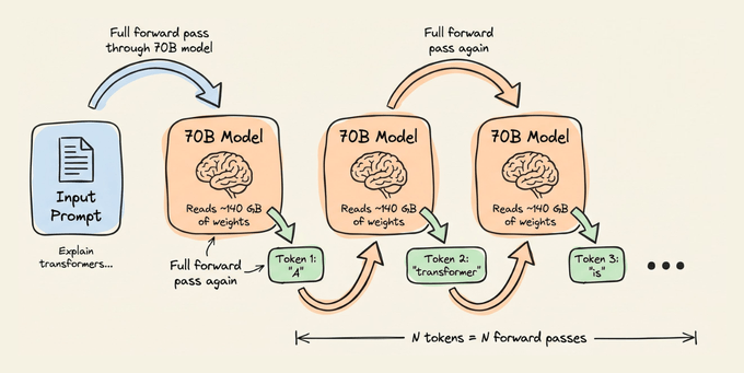
On an H100 (3.35 TB/s memory bandwidth), it would take around 42 milliseconds just to move the weights and produce exactly one token.

And here's what makes it feel particularly wasteful. The token the 70B model produces at each step is often a common, predictable word ("the", "is", "of") that even a 0.5B model could have gotten right too.

Nonetheless, you end up paying the full cost of reading 140 GB of weights to generate a token that a model 100x smaller could have produced in a fraction of the time.

Speculative decoding exploits this observation.

How speculative decoding works

Essentially, you let the small model handle the core generation process.

After a certain number of tokens (say, 5), use the large model to verify the tokens generated in a single forward pass.

Since verification processes multiple tokens at once (this is structurally identical to the prefill phase), the GPU's compute units are actually saturated rather than sitting idle waiting on memory reads.

Here's how the loop runs:

• First, a small model (e.g., Qwen2.5 0.5B) generates 5 candidate tokens autoregressively. Because it's 100x smaller than the target, this costs roughly 1-2% of a single large model forward pass.
• Then the large model (e.g., Qwen2.5 7B) processes all 5 draft tokens in a single forward pass, computing its probability distribution at each position. The draft model already produced its own distribution during drafting. Both distributions now exist side by side for comparison.
• The verification step walks through draft tokens sequentially. If the large model agrees with tokens 1, 2, and 3, but disagrees at token 4, tokens 1-3 are accepted as-is (the small model got them right), the large model replaces token 4 with its own prediction (which it already computed during the verification pass), and token 5 is discarded without evaluation.

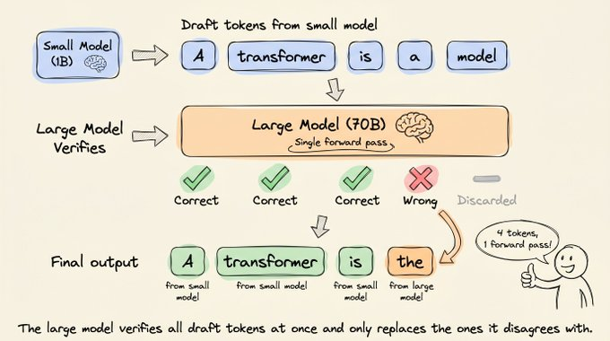
Best case, all 5 draft tokens are accepted plus one bonus token from the large model, giving you 6 tokens from just a single forward pass through the large model.

Worst case, every draft token is rejected, and you still get 1 token from the large model, which is the same as standard decoding.

The worst-case scenario is marginally more expensive than using the large model itself, but at the same time, it's also a rare incident.

Moreover, the output is mathematically identical to running the large model alone.

This is because the large model doesn't just check whether the draft tokens look right.

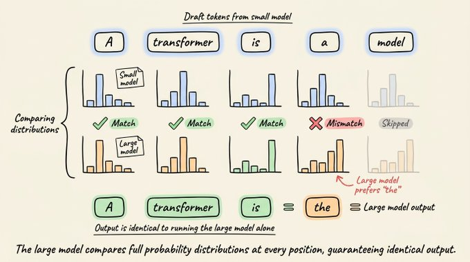
Instead, it computes its full probability distribution at every position and compares it against the small model's distribution.

Tokens are accepted only when the large model would have produced the same prediction. When it disagrees, it substitutes its own token. So every token in the final output is either directly approved or directly generated by the large model, guaranteeing an identical output distribution regardless of how good or bad the draft model is.

Implementation

Hugging Face Transformers already exposes speculative decoding as assistant_model in the generate() call.

Let's look at how to use it:

1) Load the models

from transformers import AutoModelForCausalLM, AutoTokenizer
import torch, time

target_id = "facebook/opt-6.7b"
draft_id  = "facebook/opt-125m"

tokenizer = AutoTokenizer.from_pretrained(target_id)

target = AutoModelForCausalLM.from_pretrained(target_id, torch_dtype=torch.float16, device_map="auto")
draft  = AutoModelForCausalLM.from_pretrained(draft_id,  torch_dtype=torch.float16, device_map="auto")

The target model (6.7B) is the one whose output quality we want.

The draft model (125M) is the cheap, fast one that proposes candidate tokens. Both are from the OPT family and share the exact same tokenizer, so verification happens directly at the token ID level with zero overhead.

2) Set up streaming and the input prompt

from transformers import TextStreamer
streamer = TextStreamer(tokenizer, skip_special_tokens=True)

prompt = "Explain how a transformer model processes input tokens step by step."
inputs = tokenizer(prompt, return_tensors="pt").to(target.device)

The TextStreamer prints each token to the console as it's generated. With standard decoding, tokens appear one at a time. With speculative decoding, they arrive in visible bursts whenever a batch of draft tokens gets accepted.

3) Baseline (standard decoding)

t0 = time.perf_counter()

base_out = target.generate(**inputs, max_new_tokens=200, do_sample=False, streamer=streamer)

base_time = time.perf_counter() - t0

print(f"\n⏱ Without Speculative Decoding:")
print(f"  Runtime: {base_time:.2f}s")
print(f"  Token speed: {len(base_out[0]) / base_time:.1f} tok/s")

This is the standard decode loop.

Every token requires a full forward pass through the 6.7B model. The GPU reads ~13 GB of weights from memory per token, producing one token at a time.

4) Speculative decoding (6.7B + 125M)

t0 = time.perf_counter()

spec_out = target.generate(
    **inputs, max_new_tokens=200, do_sample=False,
    assistant_model=draft,
    streamer=streamer,
)

spec_time = time.perf_counter() - t0

print(f"\n⏱ With Speculative Decoding:")
print(f"  Runtime: {spec_time:.2f}s")
print(f"  Token speed: {len(spec_out[0]) / spec_time:.1f} tok/s")
print(f"  Speedup over standard decoding: {base_time / spec_time:.2f}x")

In this specific invocation, the only addition is assistant_model=draft.

Behind the scenes, the 125M model drafts ~5 tokens autoregressively, the 6.7B model verifies all of them in a single forward pass, accepted tokens go straight to the output, and the first rejected token is replaced with the 6.7B model's own prediction. This repeats until 200 tokens are generated.

The video below shows this in action:

• The left side runs standard decoding (one token per forward pass), while the right side runs speculative decoding with the same 6.7B target model.
• The speculative run produces tokens in visible bursts as batches of draft tokens get accepted, finishing in roughly half the time with a 1.9x speedup.

For production serving, vLLM supports draft models, EAGLE, n-gram, and MTP out of the box:

from vllm import LLM, SamplingParams

llm = LLM(
    model="Qwen/Qwen2.5-72B-Instruct",
    speculative_model="Qwen/Qwen2.5-0.5B-Instruct",
    num_speculative_tokens=5,
    tensor_parallel_size=4,
)

outputs = llm.generate(["Explain speculative decoding."],
                       SamplingParams(temperature=0, max_tokens=256))

The tokenizer constraint

Traditionally, both models had to share the same tokenizer.

This is because the verification step discussed above compares the probability distributions of the large and small models at each token position.

If both models use the same tokenizer, token positions align perfectly, and the comparison is direct.

But if the tokenizers differ, the same word might get split into three tokens by one tokenizer and two tokens by another.

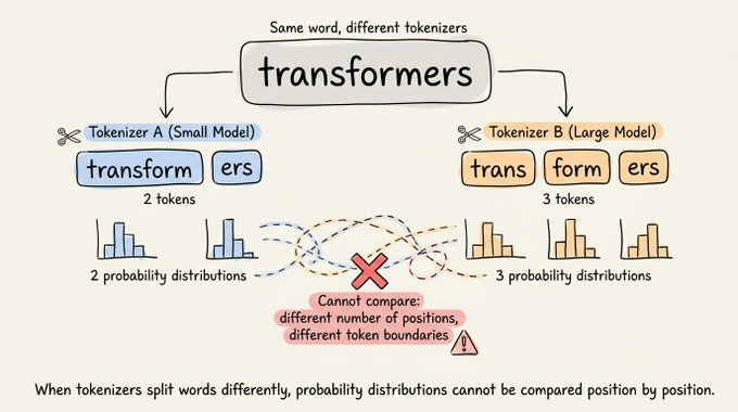
The probability distributions are now over different token spaces at different positions, and there's no meaningful way to compare them directly.

This limited speculative decoding to same-family pairs like Llama 3.2 1B with Llama 3.1 70B, Qwen2.5 0.5B with Qwen2.5 72B, etc.

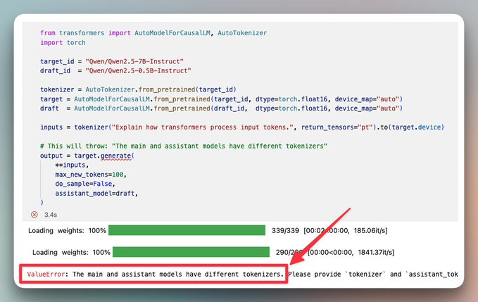
In fact, at times, even models from the same family don't always share the same tokenizer.

For instance, Qwen2.5-7B-Instruct and Qwen2.5-0.5B-Instruct have the same vocabulary:

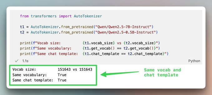
But they still differ in chat template configs, so HF Transformers framework detects this as a tokenizer mismatch:

Hugging Face shipped Universal Assisted Generation (UAG) in Transformers 4.46 (October 2024), removing that constraint entirely.

Under the hood, UAG decodes tokens generated by the small model back to text, re-encodes them with the large model's tokenizer, and aligns the sequences using longest common subsequence matching.

This lets you pair any two models regardless of tokenizer, i.e., a Qwen small model can have a Gemma large model, despite completely different tokenizers.

The tradeoff is that the same-tokenizer pairs still give better speedups (1.5-3x) compared to cross-tokenizer pairs (1.5-1.9x) because the native path skips the re-encoding overhead entirely.

One thing I noticed with speculative decoding is that even Instruct variants within the same family (e.g., Qwen2.5-7B-Instruct and Qwen2.5-0.5B-Instruct) can trigger the UAG path because Transformers compares tokenizer configs including chat templates, not just vocabulary. Using base models instead of Instruct variants avoids this and keeps you on the faster native path.

Production tradeoffs

A larger draft model (the model that generates the tokens autoregressively) improves the acceptance rate. But at the same time, it also increases drafting latency.

For instance:

• When Llama 3.2 1B was used as the draft model for Llama 3.1 70B, it achieved 2.31x speedup
• But when Llama 3.2 8B was used as the draft model, it achieved 2.08x speed up.

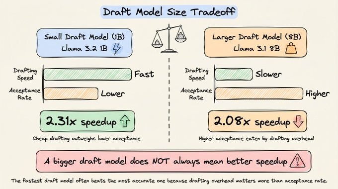
So despite its higher acceptance rate, the overall setup runs a bit slower.Sampling temperature also affects speedup.

• At temperature ~0 (greedy decoding), both models tend to agree on the top token, so acceptance rates are highest.
• As temperature increases, the probability distributions flatten, the small and large models agree less often, and more draft tokens get rejected. Creative generation tasks at high temperature see noticeably lower speedups than deterministic tasks.

We covered Temperature in LLMs here if you want to learn more →

Speculative decoding without a small model

The two-model setup has two pain points:

• You need a matched small model from the same family (for better speedups)
• Having a small model means extra GPU memory.

Several variants eliminate one or both of these problems.

1) EAGLE

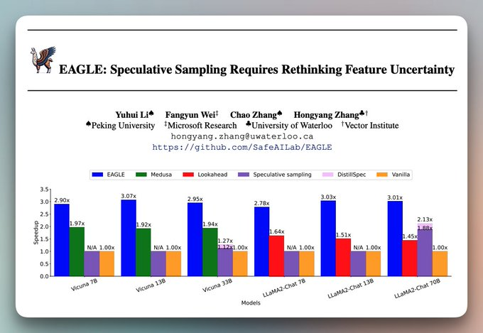
EAGLE replaces the separate draft model with a lightweight head (< 1B params) trained directly on top of the larger model.

Here's how it works step by step.

• When the large model generates a token, every layer in the transformer produces a hidden state vector for that token.
• EAGLE takes the hidden state from the second-to-last layer (the one just before the final prediction layer) because it contains rich semantic information about what the model "thinks" should come next.
• The EAGLE head is a small neural network that takes this hidden state as input and outputs a prediction for the next token, without running the full model again.

Think of it as a shortcut. Instead of passing through all the layers of a large model to predict the next token, you pass through just the EAGLE head, which is a few layers at most.

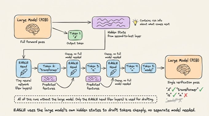
Now I want to depict how EAGLE works by depicting this particular idea that the first token is emitted from the large model, and then it uses the prediction head 2 or whatever.

Once it has drafted K tokens this way, the large model verifies all of them in a single forward pass, exactly like standard speculative decoding.

The key advantage is that these predictions are grounded in the large model's own internal representations, not from a separate, smaller model that was trained independently.

This is also why there's no tokenizer issue since the EAGLE head lives inside the target model's architecture and operates in the same token space.

2) Medusa

Instead of drafting tokens one after another, it predicts multiple future tokens simultaneously from a single forward pass.

Under the hood, Medusa attaches several small prediction heads to the large model, each responsible for a different position ahead.

• Head 1 predicts what the next token will be.
• Head 2 predicts what the token two positions ahead will be.
• Head 3 predicts three positions ahead, and so on.

All these heads run in parallel during a single forward pass of the large model. So from one pass, you get predictions for the next 5 positions at once, not just one.

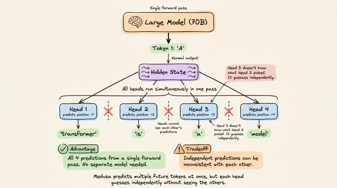
As expected, one key problem is that each head makes its prediction independently. Head 2 doesn't know what Head 1 predicted.

In normal autoregressive generation, the prediction for token 3 depends on what token 2 actually was.

Medusa can't do that because all heads run at the same time. So head 3 might predict "model" assuming token 2 was "language," while head 2 actually predicted "learning."

The candidates can be inconsistent with each other, which lowers acceptance rates compared to EAGLE, where each drafted token is conditioned on the previous one.

The upside is that there's no separate model and extra memory required for a drafter. The heads are also tiny (a few linear layers each), so the overhead per forward pass is minimal.

3) Self-speculative decoding

This method requires no separate model, additional heads, or training at all.

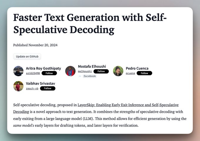
It uses the large model itself as both the drafter and the verifier. The idea relies on how transformers are structured.

A 70B model might have 80 layers, and each layer refines the prediction from the previous one.

For many tokens, the model's early layers (say, the first 12 out of 80) already have enough information to make the right prediction.

The remaining 68 layers just confirm what the early layers already figured out.

Self-speculative decoding exploits this observation.

During drafting, the model runs only its first N layers and exits early with a prediction.

It does this K times to produce K draft tokens.

Then, during verification, the full model (all 80 layers) runs a single forward pass over all K tokens to check which ones the early exit got right.

For easy, predictable tokens, the early layers are usually sufficient, and those tokens get accepted.

For harder tokens where the later layers would have changed the prediction, the draft gets rejected, and the full model's output is used instead.

The speedups are more modest (1.3-1.8x) because the drafter isn't a separate cheap model.

It's still the same large model, just running fewer layers. But the tradeoff is that you need absolutely nothing extra, like a second model to download, heads to train, or extra GPU memory.

4) Diffusion-based drafting

This method addresses a fundamental inefficiency in all the methods above.

Even with EAGLE, Medusa, or a separate draft model, the drafting process itself is still autoregressive. The drafter generates token 1, then token 2, then token 3, one at a time.

The draft model is faster because it's smaller, but it's still sequential.

Diffusion models work completely differently.

Instead of predicting one token at a time, a diffusion model starts with a block of random noise tokens and iteratively refines all of them in parallel.

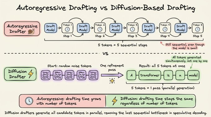
In just a few refinement steps, the entire block converges to coherent text. So where an autoregressive drafter generates 8 tokens in 8 sequential steps, a diffusion drafter generates all 8 in a single forward pass (or a small fixed number of passes regardless of how many tokens you want).

DFlash takes this idea and makes it practical for speculative decoding. Instead of training a standalone diffusion model from scratch (which would be large and expensive), it trains a small diffusion head that takes the target model's hidden states as conditioning input, similar to how EAGLE uses the target model's representations.

The diffusion head then generates an entire draft block in parallel, conditioned on what the large model has already computed.

This way, the drafting cost no longer scales with the number of tokens you want to propose.

An autoregressive drafter that proposes 16 tokens needs 16 sequential steps. A diffusion drafter proposes all 16 in one pass.

The speed up is evident from the video below:

The verification step remains the same as standard speculative decoding. The large model checks all proposed tokens in a single forward pass and accepts or rejects them.

The only difference is how the draft tokens were generated, i.e., in parallel via diffusion rather than sequentially via autoregression.

Speculative decoding is converging toward single-model solutions where the draft capability is built into the target model itself.

For most production setups today, the two-model approach with a same-family drafter remains the simplest path to 2-3x speedups.

But regardless of which variant you use, all of them rely on KV caching internally to work efficiently.

The draft model maintains its own KV cache, so each draft token builds on the previous one cheaply.

The target model's verification pass extends its KV cache with accepted tokens, so the next iteration doesn't recompute anything for them.

Without KV caching, both drafting and verification would be far more expensive, and the speedups from speculative decoding would largely disappear.

In other words, speculative decoding reduces how many forward passes you need, and KV caching makes each of those forward passes efficient. They work together, not as alternatives.

As further reading:

We covered the mechanics of LLM inference (prefill and decode phases, KV caching, speculative decoding, batching, and optimization techniques that improve latency and throughput here in the LLMOps course →

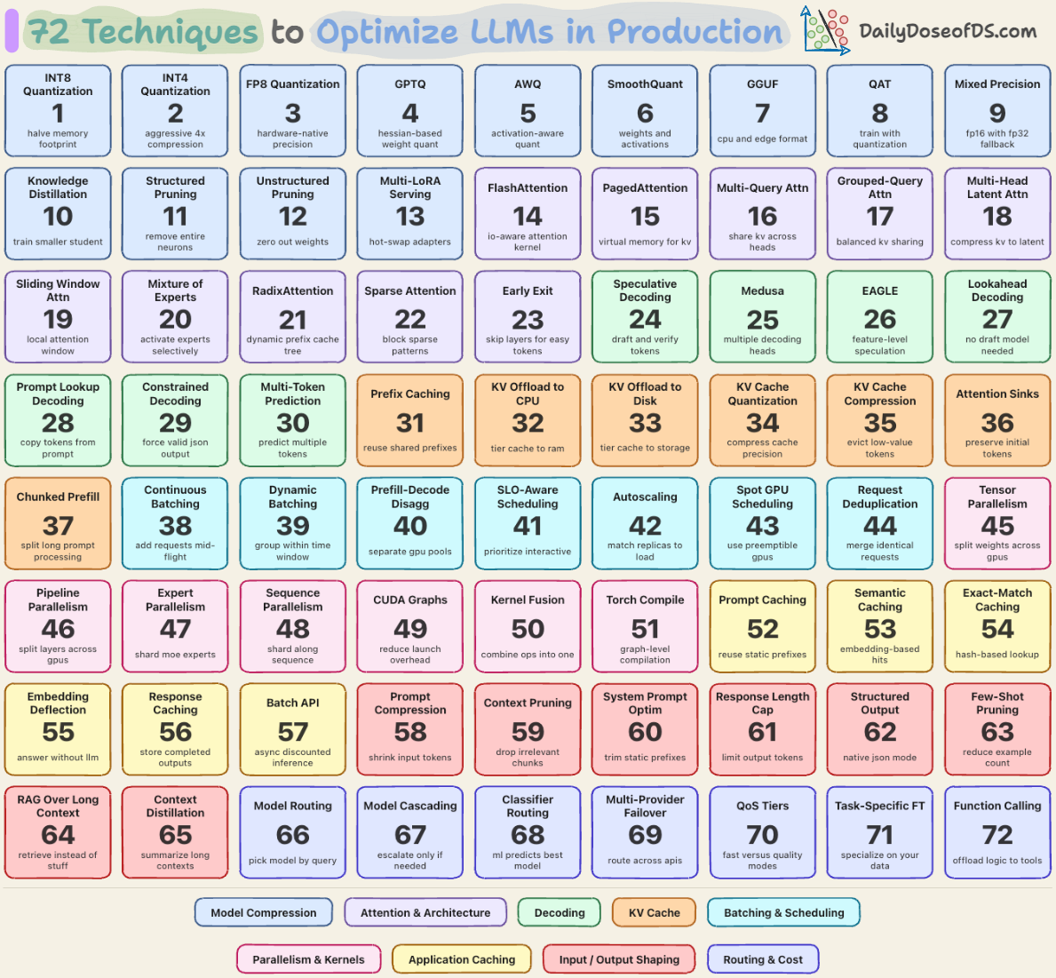
And we covered 72 techniques to optimize LLMs in production here →

Thanks for reading!