Mixed Precision Training

TODAY’S DAILY DOSE OF DATA SCIENCE

Mixed Precision Training

Typical deep learning libraries are really conservative when it comes to assigning data types.

The data type assigned by default is usually 64-bit or 32-bit, when there is also scope for 16-bit, for instance. This is also evident from the code below:

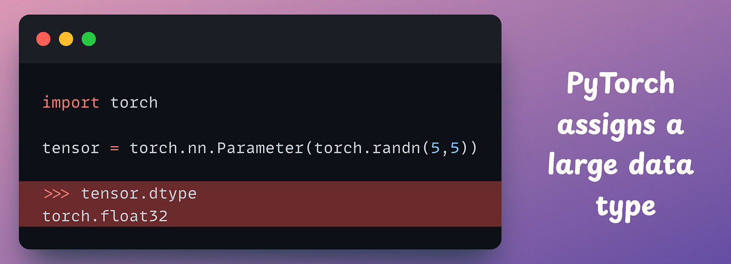
As a result, we are not entirely optimal at efficiently allocating memory.

Of course, this is done to ensure better precision in representing information.

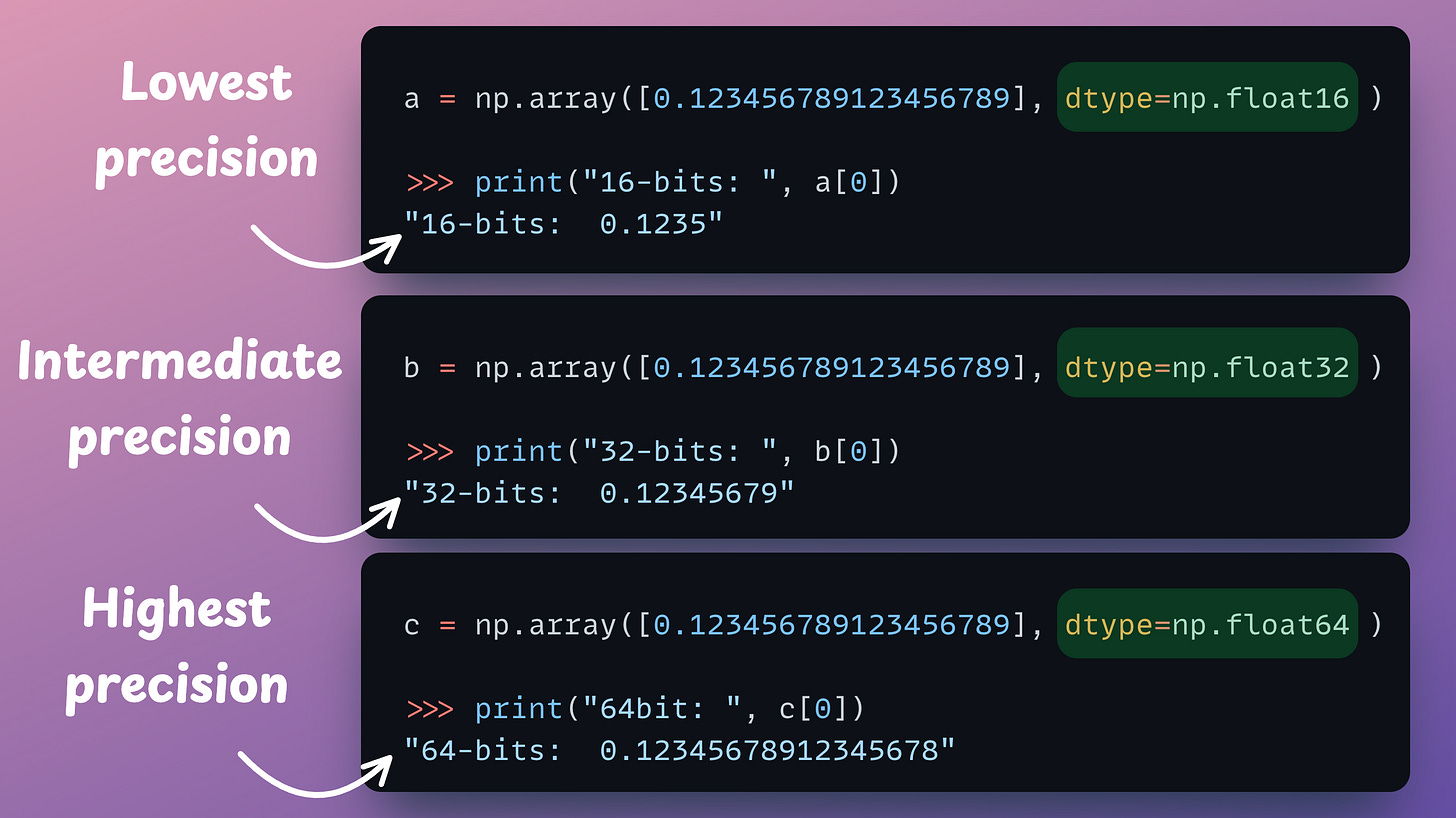
However, this precision always comes at the cost of additional memory utilization, which may not be desired in all situations.

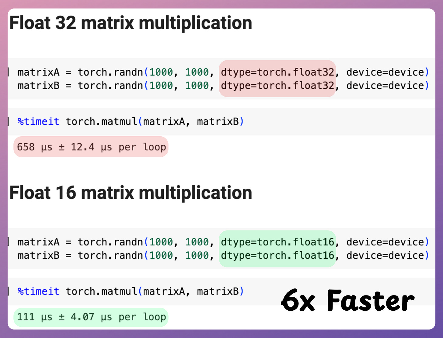
In fact, it is also observed that many tensor operations, especially matrix multiplication, are much faster when we operate under smaller precision data types than larger ones, as demonstrated below:

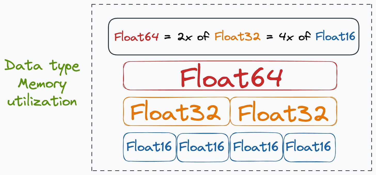
Moreover, since float16 is only half the size of float32, its usage reduces the memory required to train the network.

This also allows us to train larger models, train on larger mini-batches (resulting in even more speedup), etc.

Mixed precision training is a pretty reliable and widely adopted technique in the industry to achieve this.

As the name suggests, the idea is to employ lower precision float16 (wherever feasible, like in convolutions and matrix multiplications) along with float32 — that is why the name “mixed precision.”

This is a list of some models I found that were trained using mixed precision:

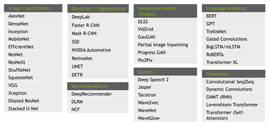
It’s pretty clear that mixed precision training is much more popularly used, but we don’t get to hear about it often.

Before we get into the technical details…

From the above discussion, it must be clear that as we use a low-precision data type (float16), we might unknowingly introduce some numerical inconsistencies and inaccuracies.

To avoid them, there are some best practices for mixed precision training that I want to talk about next, along with the code.

Mixed precision training in PyTorch and Best Practices

Leveraging mixed precision training in PyTorch requires a few modifications in the existing network training implementation.

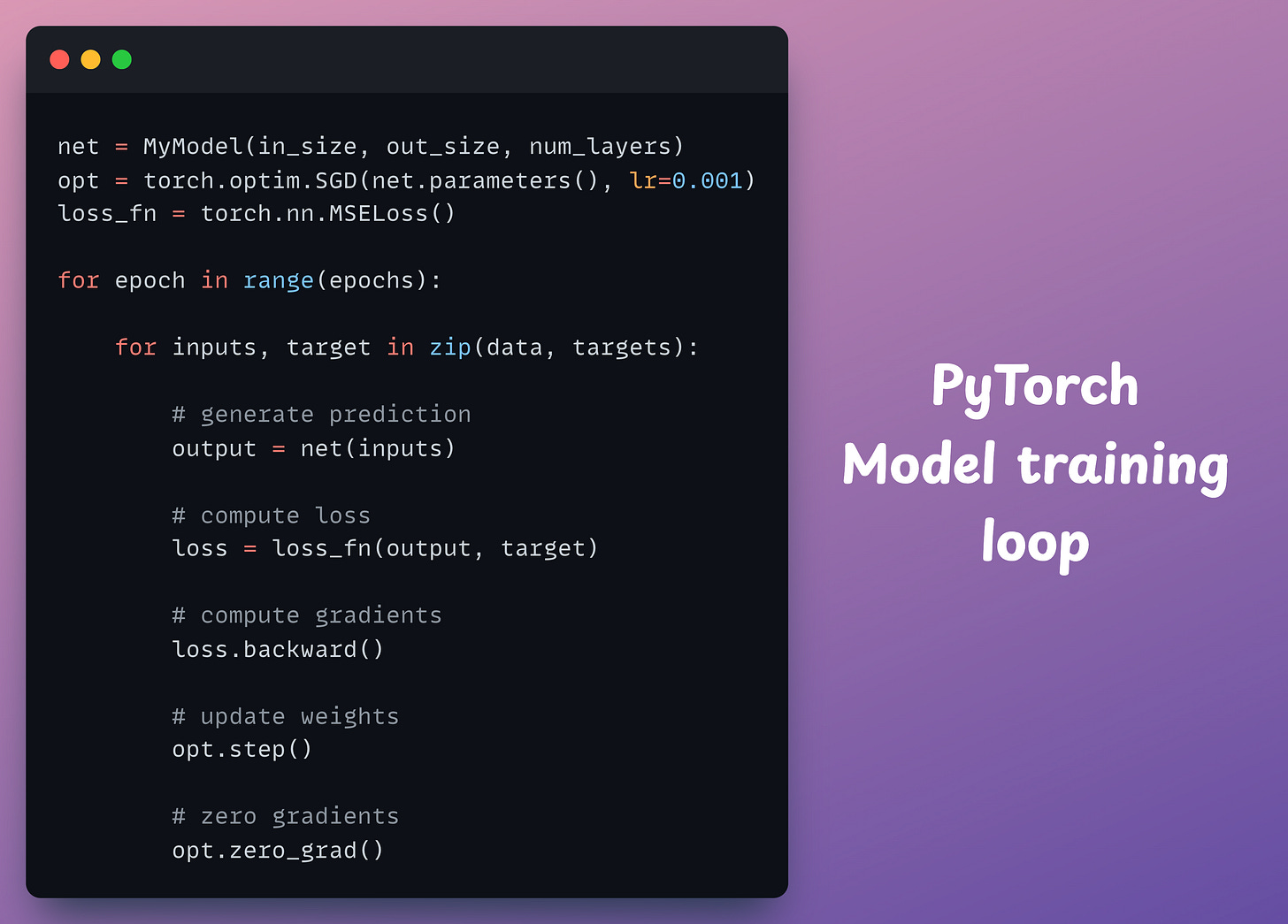
Consider this is our current PyTorch model training implementation:

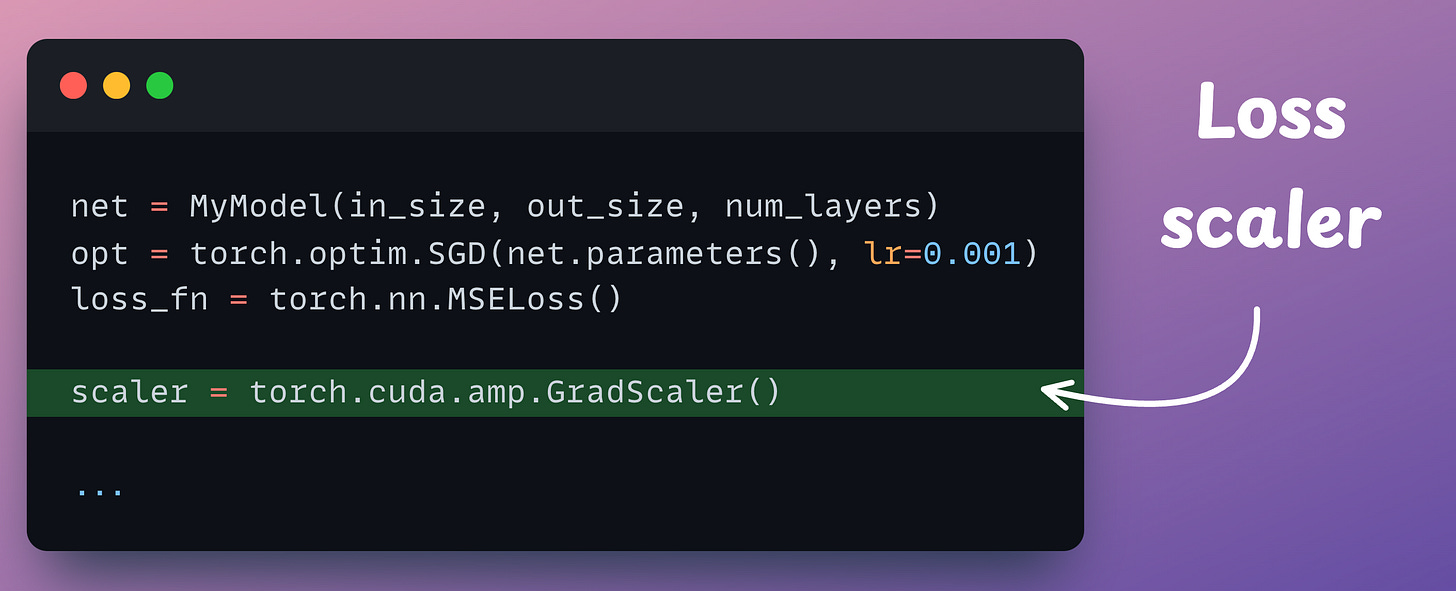
The first thing we introduce here is a scaler object that will scale the loss value:

We do this because, at times, the original loss value can be so low, that we might not be able to compute gradients in float16 with full precision.

Such situations may not produce any update to the model’s weights.

Scaling the loss to a higher numerical range ensures that even small gradients can contribute to the weight updates.

But these minute gradients can only be accommodated into the weight matrix when the weight matrix itself is represented in high precision, i.e., float32.

Thus, as a conservative measure, we tend to keep the weights in float32.

That said, the loss scaling step is not entirely necessary because, in my experience, these little updates typically appear towards the end stages of the model training.

Thus, it can be fair to assume that small updates may not drastically impact the model performance.

But don’t take this as a definite conclusion, so it’s something that I want you to validate when you use mixed precision training.

Moving on, as the weights (which are matrices) are represented in float32, we can not expect the speedup from representing them in float16, if they remain this way:

To leverage these flaot16-based speedups, here are the steps we follow:

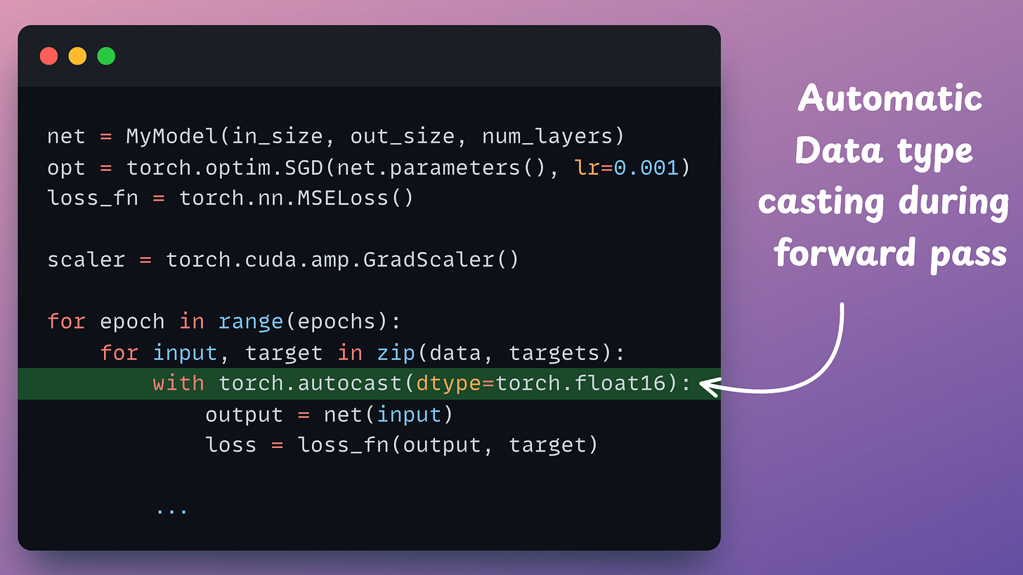
1. We make a float16 copy of weights during the forward pass.
2. Next, we compute the loss value in float32 and scale it to have more precision in gradients, which works in float16.
   1. The reason we compute gradients in float16 is because, like forward pass, gradient computations also involve matrix multiplications.
   2. Thus, keeping them in float16 can provide additional speedup.
3. Once we have computed the gradients in float16, the heavy matrix multiplication operations have been completed. Now, all we need to do is update the original weight matrix, which is in float32.
4. Thus, we make a float32 copy of the above gradients, remove the scale we applied in Step 2, and update the float32 weights.
5. Done!

The mixed-precision settings in the forward pass are carried out by the torch.autocast() context manager:

Now, it’s time to handle the backward pass.

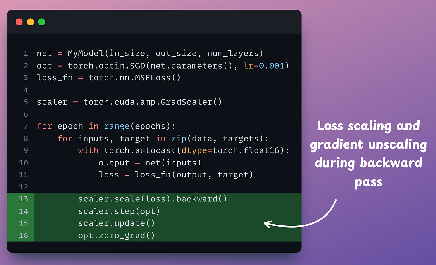
• Line 13 → scaler.scale(loss).backward(): The scaler object scales the loss value and backward() is called to compute the gradients.
• Line 14 → scaler.step(opt): Unscale gradients and update weights.
• Line 15 → scaler.update(): Update the scale for the next iteration.
• Line 16 → opt.zero_grad(): Zero gradients.

Done!

The efficacy of mixed precision scaling over traditional training is evident from the image below:

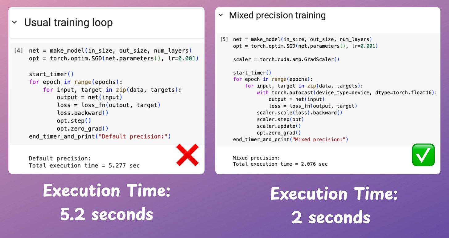
Mixed precision training is over 2.5x faster than conventional training.

Isn’t that impressive?

👉 Over to you: What are some other reliable ways to speed up machine learning model training?

EXTENDED PIECE #1

Beyond grid and random search

There are many issues with Grid search and random search.

• They are computationally expensive due to exhaustive search.
• The search is restricted to the specified hyperparameter range. But what if the ideal hyperparameter exists outside that range?
• They can ONLY perform discrete searches, even if the hyperparameter is continuous.

Bayesian optimization solves this.

It’s fast, informed, and performant, as depicted below:

Learning about optimized hyperparameter tuning and utilizing it will be extremely helpful to you if you wish to build large ML models quickly.

Learn Bayesian Optimization from scratch here →

EXTENDED PIECE #2

Beyond linear regression

Linear regression makes some strict assumptions about the type of data it can model, as depicted below.

Can you be sure that these assumptions will never break?

Nothing stops real-world datasets from violating these assumptions.

That is why being aware of linear regression’s extensions is immensely important.

Generalized linear models (GLMs) precisely do that.

They relax the assumptions of linear regression to make linear models more adaptable to real-world datasets.

Learn Generalized linear models from scratch here →