Sklearn Models are Not Deployment Friendly! Supercharge Them With Tensor Computations.

The scikit-learn project has possibly been one of the most significant contributions to the data science and machine learning community for building traditional machine learning (ML) models.

Personally speaking, it’s hard to imagine a world without sklearn.

However, things get pretty concerning if we intend to deploy sklearn-driven models in real-world systems.

Let’s understand why.

Limitations of Sklearn models in deployment

Scikit-learn models are primarily built on top of NumPy, which, of course, is a fantastic and high-utility library for numerical computations in Python.

Yet, contrary to common belief, NumPy isn’t as optimized as one may hope to have in real-world ML systems.

One substantial reason for this is that NumPy can only run on a single core of a CPU.

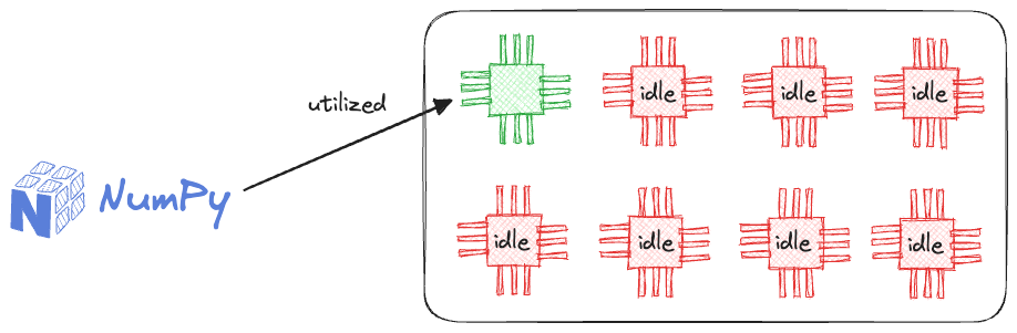
This provides massive room for improvement as there is no parallelization support in NumPy (yet), and it naturally becomes a big concern for data teams to let NumPy drive their production systems.

While traditional ML models do perform well on tabular datasets, but as we discussed in a recent blog on model compression: “Typically, when we deploy any model to production, the specific model that gets shipped to production is NOT solely determined based on performance. Instead, we must consider several operational metrics that are not ML-related.”

Another major limitation is that scikit-learn models cannot natively run on Graphics Processing Units (GPUs).

Having GPU support in deployment matters because real-world systems often demand lightning-fast predictions and processing.

However, as discussed above, sklearn models are primarily driven by NumPy, which, disappointingly, can only run on a single core of a CPU. In this context, it is unlikely to have GPU support anytime soon.

In fact, this is also mentioned on Sklearn’s FAQ page:

• Question: Will you add GPU support?
• Answer: No, or at least not in the near future. The main reason is that GPU support will introduce many software dependencies and introduce platform-specific issues. scikit-learn is designed to be easy to install on a wide variety of platforms.

Further, they mention that “Outside of neural networks, GPUs don’t play a large role in machine learning today, and much larger gains in speed can often be achieved by a careful choice of algorithms.”

I don’t entirely agree with this specific statement.

Consider the enterprise space. Here, the data is primarily tabular. Classical ML techniques such as linear models and tree-based ensemble methods are frequently used to model the tabular data.

In fact, when you have tons of data to model, there’s absolutely no reason to avoid experimenting with traditional ML models first.

Yet, in the current landscape, one is often compelled to train and deploy deep learning-based models just because they offer optimized matrix operations using tensors.

We see a clear gap here.

Thus, in this article, let’s learn a couple of techniques today:

• How do we run traditional ML models on large datasets?
• How do we integrate GPU support with traditional ML models in deployment systems?
  • While there is no direct way to do this, we must (somehow) compile our machine-learning model to tensor operations, which can be loaded on a GPU for acceleration. We’ll discuss this in the article shortly.

But before that, we must understand a few things.

More specifically:

• What are tensors?
• How are tensors different from a traditional NumPy array?
• Why are tensor computations faster than NumPy operations, and why are tensor operations desired?

Let’s begin!

What are tensors?

Many often interpret tensors as a complicated and advanced concept in deep learning.

However, it isn’t.

The only thing that is ever there to understand about Tensors is that, like any NumPy array, Tensors are just another data structure to store multidimensional data.

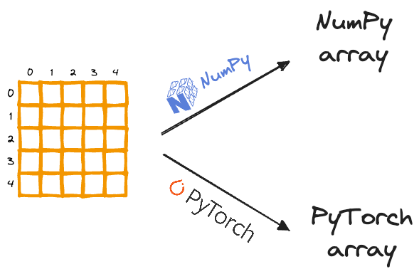
• When we use NumPy to store numerical data, we create a NumPy array — NumPy’s built-in data structure.
• When we use PyTorch (for instance) to store numerical data, we create a Tensor — PyTorch’s built-in data structure.

That’s it.

Tensor, like NumPy array, is just another data structure.

Why Tensors?

Now, an obvious question at this point is:

Why create another data structure when NumPy arrays do the exact same thing of storing multidimensional data, and they are very well integrated with other scientific Python libraries?

There are multiple reasons why PyTorch decided to develop a new data structure.

Limitation #1) NumPy isn’t parallelized

NumPy undoubtedly offers:

• extremely fast, and
• optimized operations.

This happens through its vectorized operations.

Simply put, vectorization offers run-time optimization:

• when dealing with a batch of data together…
• …by avoiding native Python for-loops (which are slow).

But as discussed earlier in this article, NumPy DOES NOT support parallelism.

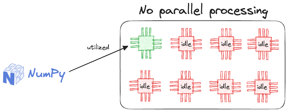
Thus, even though its operations are vectorized, every operation is executed in a single core of the processing unit.

This provides further scope for run-time improvement.

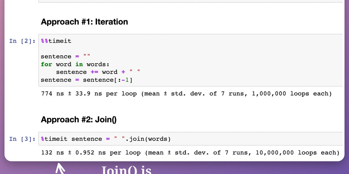
Of course, there are open-source libraries like Numexpr that address this limitation by providing a fast evaluator for NumPy expression using:

• Multi-threading:
  • It is a parallel computing technique that allows a program to execute multiple threads (smaller units of a process) concurrently.
  • In the context of NumPy and libraries like Numexpr, multi-threading accelerates mathematical and numerical operations by dividing the computation across multiple CPU cores.

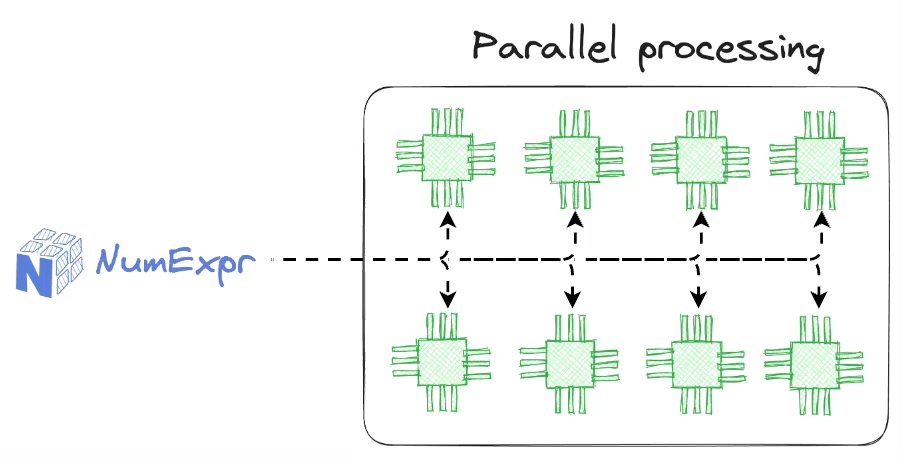
• This approach is particularly effective when you have a multi-core CPU, as it leverages the available cores for parallelism, leading to faster computation.
• Just-in-time (JIT) compilation:
  • JIT compilation is a technique used to improve the run-time performance of code by compiling it at run-time, just before execution.

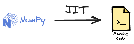
• In the context of Numexpr (and similar libraries, JIT compilation involves taking a NumPy expression or mathematical operation and dynamically generating machine code specific to the operation.
• As a result, JIT-compiled code can run much faster than equivalent pure Python code because it is optimized for the specific operation and can make use of low-level hardware features.

The speedup offered by Numexpr is evident from the image below.

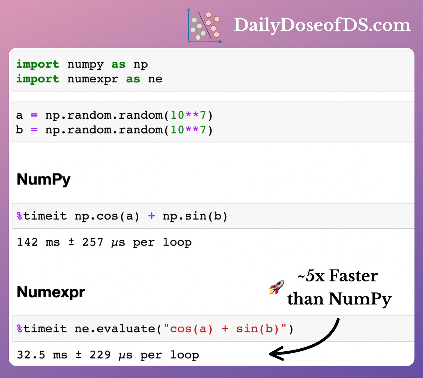
According to Numexpr’s documentation, depending upon the complexity of the expression, the speed-ups can range from 0.95x to 20x.

Nonetheless, the biggest problem is that Numexpr can only speed up element-wise operations on NumPy arrays.

This includes:

• Element-wise sum/multiplication etc.
• Element-wise transformations like sin, log, etc.
• and more.

But Numexpr has no parallelization support for matrix multiplications, which, as you may already know, are the backbone of deep learning models.

This problem gets resolved in PyTorch tensors as they offer parallelized operations.

An important point to note:

• GPU parallelization:
  • If you're working with PyTorch tensors on a GPU (using CUDA), the matrix multiplication operation is highly parallelized across the numerous cores of the GPU.
  • Modern GPUs consist of thousands of cores designed for parallel computation.
  • When you perform a matrix multiplication on a GPU, these cores work together to compute the result much faster than a CPU could.
• CPU Parallelization:
  • The extent of parallelization on a CPU may depend on the CPU’s architecture.
  • All CPUs these days have multiple cores, and PyTorch is optimized to utilize these cores efficiently for matrix operations.
  • While it may not be as parallel as a GPU, you can still expect significant speed improvements over performing the operation in pure Python.

We can also verify experimentally:

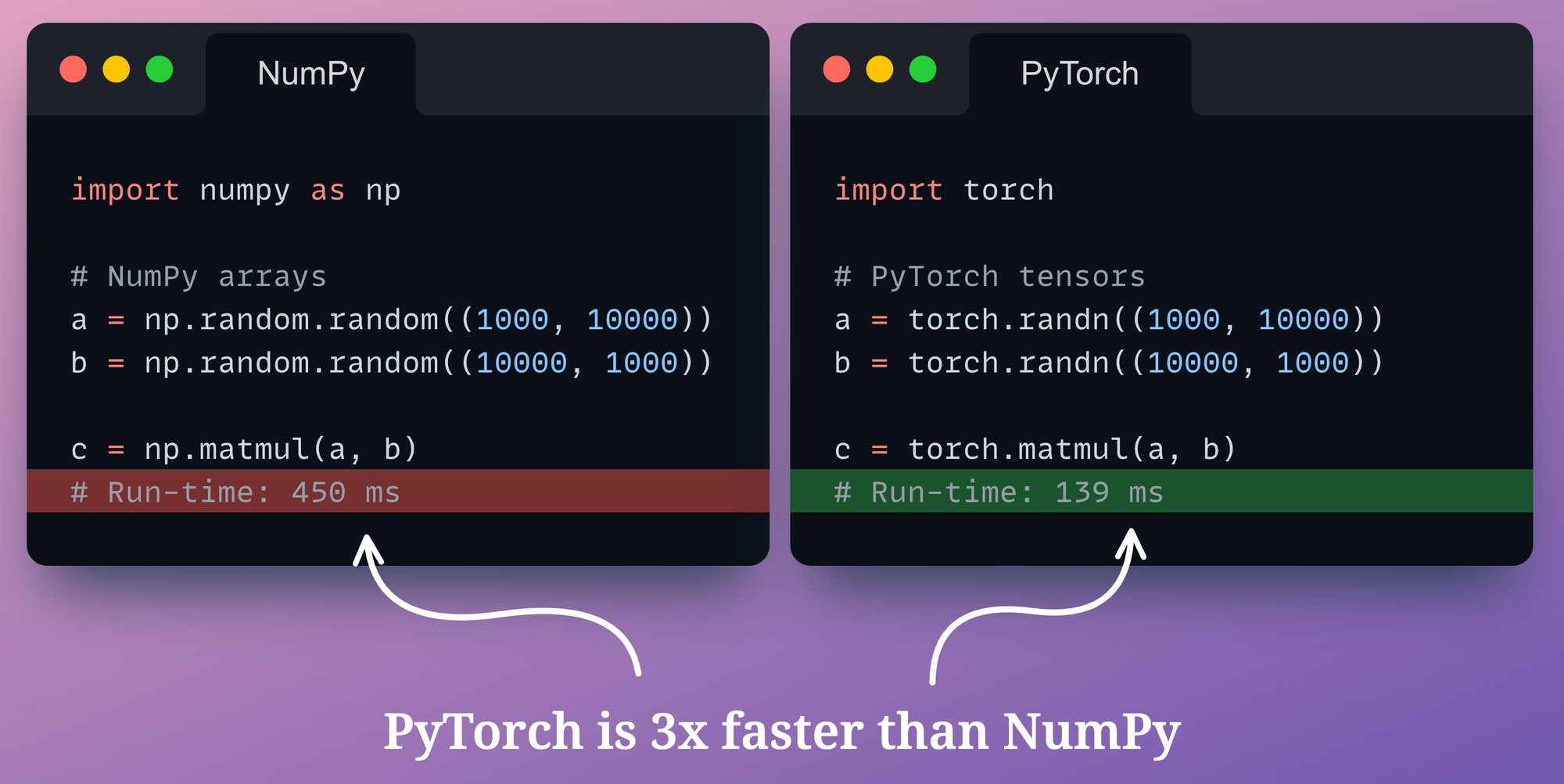
• On the left, we create two random NumPy arrays and perform matrix multiplication using np.matmul() method.
• On the right, we create two random PyTorch tensors and perform matrix multiplication using torch.matmul() method.

As depicted above, PyTorch is over three times faster than NumPy, which is a massive speed-up.

This proves that PyTorch provides highly optimized vector operations, which the neural network can benefit from, not only during forward pass but backpropagation as well.

In fact, here’s another reason why tensor operations in PyTorch are faster.

See, as we all know, NumPy is a general-purpose computing framework that is designed to handle a wide range of numerical computations across various domains, not limited to just deep learning or machine learning.

In fact, NumPy is not just used by data science and machine learning practitioners, but it is also widely used in various scientific and engineering fields for tasks such as signal processing, image analysis, and simulations in physics, chemistry, and biology.

It’s so popular in Biological use cases that a bunch of folks extended the NumPy package to create BioNumPy:

BioNumPy: Fast and easy analysis of biological data with Python

Python is a popular and widespread programming language for scientific computing, in large part due to the powerful array programming library NumPy, which makes it easy to write clean, vectorized and efficient code for handling large datasets. A challenge with using array programming for biological…

bioRxivView ORCID Profile

While its versatility is a key strength, it also means that NumPy’s internal optimizations are geared toward a broad spectrum of use cases.

On the other hand, PyTorch is purposely built for deep learning and tensor operations.

This specialized focus allows PyTorch to implement highly tuned and domain-specific optimizations for tensor computations, including matrix multiplications, convolutions, and more.

These optimizations are finely tuned to the needs of deep learning, where large-scale matrix operations are fundamental.

Being niched down to a specific set of users allowed PyTorch developers to optimize tensor operations, including matrix multiplication to a specific application — deep learning.

If you want another motivating example, we discussed this in the newsletter here:

What Makes The Join() Method Blazingly Faster Than Iteration?

A reminder to always prefer specific methods over a generalized approach.

Daily Dose of Data ScienceAvi Chawla

In a gist, the core idea is that the more specific we get, the better we can do compared to a generalized solution.

Limitation #2) NumPy cannot track operations

Deep learning is all about a series of matrix operations applied layer after layer to generate the final output.

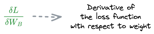
For instance, consider the following neural network for regression:

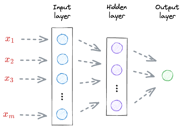
• First, the input received at the input layer $(x_1, x_2, \cdots, x_m)$ is transformed by a set of weights $(W_A)$ and an activation function to get the output of the hidden layer.
• Next, the output of the hidden layer is further transformed by a set of weights $(W_B)$ to get the final output (t).

If we were to use NumPy to represent input, weights, and layer outputs, it would be impossible to tell how a specific array was computed.

For instance, consider the two NumPy arrays arr1 and arr2 below:

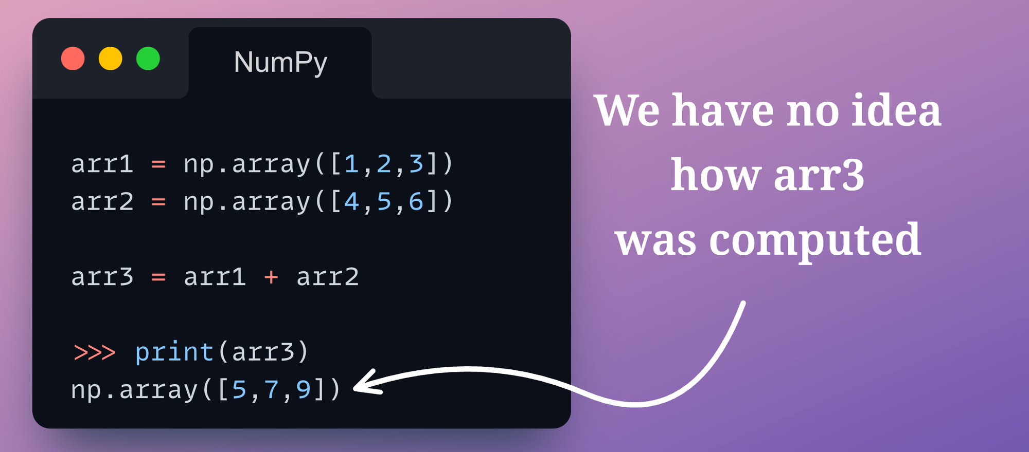
The NumPy array arr3 holds no information about how it was computed.

In other words, as long as we don’t manually dig into the code, we can never tell:

• What were the operands?
• What was the operator?

But why do we even care about that information?

See, as long as we are only doing a forward pass in a neural network, we don’t care which specific operation and which arrays generated a particular layer output. We only care about the output in that case.

But that’s not how neural networks are trained, are they?

To train a neural network, we must run backpropagation.

To run backpropagation, we must compute gradients to update the weights.

And to compute gradients of a layer’s weights, we must know the specific arrays that were involved in that computation.

For instance, consider the above neural network again:

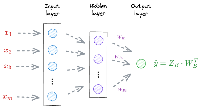
To update the weights $W_B$, we must compute the gradient $\Large \frac{\delta L}{\delta W_B}$.

The above gradient depends on the loss value $L$, which in turn depends on $\hat y$.

Thus, we must know the specific vectors that were involved in the computation of $\hat y$.

While this is clear from the above network:

• What if we add another layer?
• What if we change the activation function?
• What if we add more neurons to the layer?
• What if we were to compute the gradient of weight in an earlier layer?

All this can get pretty tedious to manage manually.

However, if (somehow) we can keep track of how each tensor was computed, what operands were involved, and what the operator was, we can simplify gradient computation.

A computational graph helps us achieve this.

Simply put, a computational graph is a directed acyclic graph representing the sequence of mathematical operations that led to the creation of a particular tensor.

During network training, PyTorch forms this computational graph during the forward pass.

For instance, the computational graph for a dummy neural network is shown below:

• First, we perform a matrix multiplication between the input $X$ and the weights $W_A$ to get the output activations $Z_B$ (we are ignoring any activation functions for now).
• Next, we perform a matrix multiplication between the output activations $Z_B$ and the weights $W_B$ to get the network output $Z_C$.

During backpropagation, PyTorch starts scanning the computational graph backward, i.e., from the output node, iteratively computes the gradients, and updates all the weights.

The program that performs all the gradient computation is called PyTorch Autograd.

Limitation #3) NumPy computations cannot run on hardware accelerators

Large deep learning models demand plenty of computational resources for speeding up model training.

However, NumPy operations are primarily designed to run on the Central Processing Unit (CPU), which is the general-purpose processor in most computers.

While CPUs are versatile and suitable for many tasks, they do not provide the speed and parallel processing capabilities needed for large-scale numerical computations, especially in the context of modern deep learning and scientific computing.

On a side note, if you genuinely want to run NumPy-like computation on a GPU, CuPy is an open-source NumPy alternative that you may try.

It’s a NumPy-compatible array library for GPU-accelerated computing.

The syntax of CuPy is quite compatible with NumPy. To use GPU, you just need to replace the following line of your code:

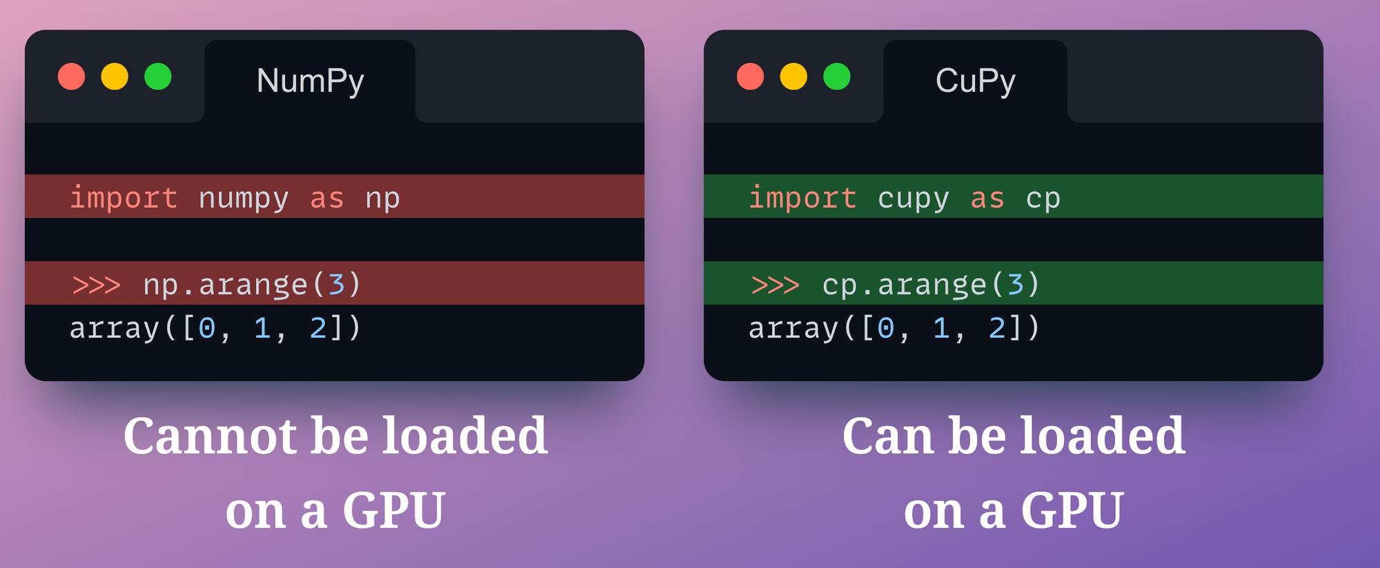
Nonetheless, the issue of not being able to track how each array was computed still exists with CuPy.

Thus, even if we wanted to, we could not use CuPy as an alternative to NumPy.

In fact, CuPy, like NumPy, is also a general-purpose scientific computation library. So any deep learning-specific optimizations are still not up to the mark.

These limitations prompted PyTorch developers to create a new data structure, which addressed these limitations.

This also suggests that by somehow compiling machine learning models to tensor computations, we can leverage immense inference speedups.

Before getting into those details, let’s understand how we can train sklearn models on large datasets on a CPU.

Sklearn models on big datasets

So far, we have spent plenty of time understanding the motivation for building traditional ML models on large datasets.

As sklearn can only utilize CPU, using it for large datasets is still challenging.

Yet, there’s a way.

We know that sklearn provides a standard API across each of its machine learning model implementations.

• Train the model using model.fit().
• Predict the output using model.predict().
• Compute the accuracy using model.score().
• and more.

However, the problem with training a model this way is that the sklearn API expects the entire training data at once.

This means that the entire dataset must be available in memory to train the model.

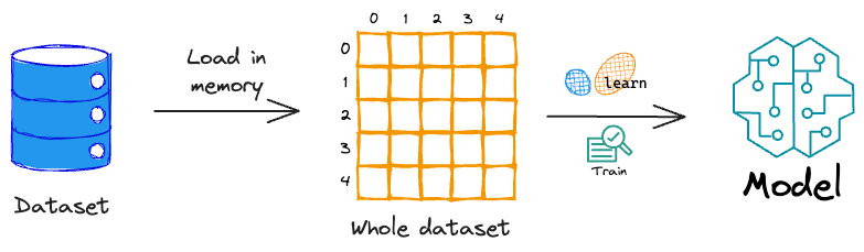
But what if the dataset itself is large enough to load in memory? These are called out-of-memory datasets.

In fact, even if we can somehow barely load the dataset in memory, it might be difficult to train the model because every model requires some amount of computations, which, of course, will consume memory.

Thus, there’s a high possibility that the program (or Jupyter kernel) may crash.

Nonetheless, there’s a solution to this problem.

In situations where it’s not possible to load the entire data into the memory at once, we can load the data in chunks and fit the training model for each chunk of data.

This is also called incremental learning and sklearn, considerately, provides the flexibility to do so.

More specifically, Sklearn implements the partial_fit() API for various algorithms, which offers incremental learning.

As the name suggests, the model can learn incrementally from a mini-batch of instances. This prevents limited memory constraints as only a few instances are loaded in memory at once.

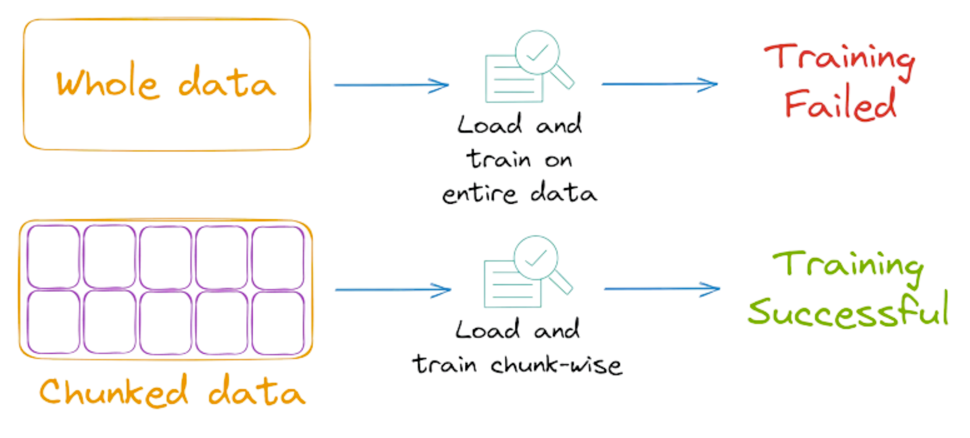
What’s more, by loading and training on a few instances at a time, we can possibly speed up the training of sklearn models.

Why?

Usually, when we use the model.fit(X, y) method to train a model in sklearn, the training process is vectorized but on the entire dataset.

While vectorization provides magical run-time improvements when we have a bunch of data, it is observed that the performance may degrade after a certain point.

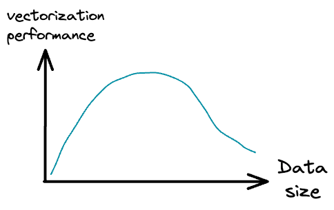
Thus, by loading fewer training instances at a time into memory and applying vectorization, we can get a better training run-time.

Let’s see this in action!

First, let’s create a dummy classification dataset with:

• 20 Million training instances
• 5 features
• 2 classes

We will use the make_classification() method from sklearn to do so:

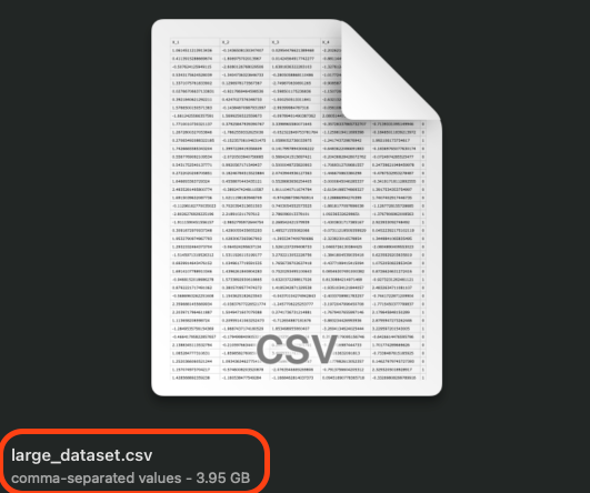
After creating a Pandas DataFrame and exporting it to a CSV, the dataset occupies roughly 4 GBs of local storage space:

We train a SGDClassifier model using sklearn on the entire dataset as follows:

The above training takes about $251$ seconds.

Next, let’s train the same model using the partial_fit() API of sklearn.

Here’s what we shall do:

• Load data from the CSV file large_dataset.csv in chunks
  • We can do this by specifying the chunksize parameter in pd.read_csv() method.
  • Say chunksize=400000, then this would mean that Pandas will only load four lakh rows at a time in memory.
• After loading a specific chunk, we will invoke the partial_fit() API on the SGDClassifier model.

This is implemented below:

The training time is reduced by ~8 times, which is massive.

This validates what we discussed earlier:

While vectorization provides magical run-time improvements when we have a bunch of data, it is observed that the performance may degrade after a certain point. Thus, by loading fewer training instances at a time into memory and applying vectorization, we can get a better training run-time.

Of course, we must also compare the model coefficients and prediction accuracy of the two models.

The following visual depicts the comparison between model_full and model_chunk:

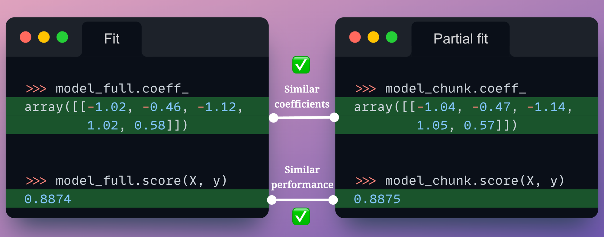
Both models have similar coefficients and similar performance.

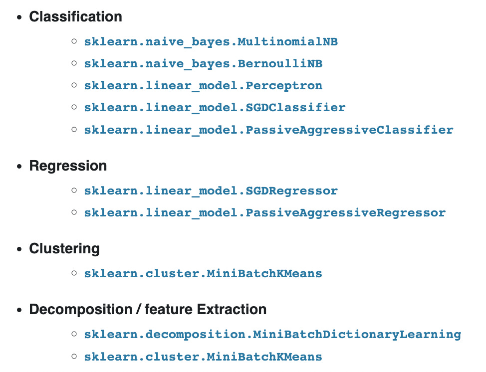
Having said that, it is also worth noting that not all sklearn estimators implement the partial_fit() API.

Here's the list of models that do:

Once we have trained our sklearn model (either on a small dataset or large), we may want to deploy it.

However, as discussed earlier, sklearn models are backed by NumPy computations, so they can only run on a single core of a CPU.

Thus, in a deployment scenario, this can lead to suboptimal run-time performance.

Nonetheless, it is possible to compile many sklearn models to tensor operations, which can be loaded on a GPU to gain immense speedups.

Let’s understand how.

Sklearn model inference using a GPU