5 LLM Quantization Techniques

A 70B parameter model in FP16 requires 140GB of memory for weights alone.

That exceeds any single GPU available today:

• An H100 carries 80GB
• An RTX 4090 carries 24GB

So serving the model in half precision means multi-GPU setups and tensor parallelism before the first token is generated.

Quantization reduces this footprint by storing weights in lower bits.

The standard scheme maps each weight from FP16 onto a small integer grid: compute the dynamic range of the tensor, divide it into 2^b levels (16 levels at 4-bit), round each weight to the nearest level, and store a scale factor to dequantize during inference.

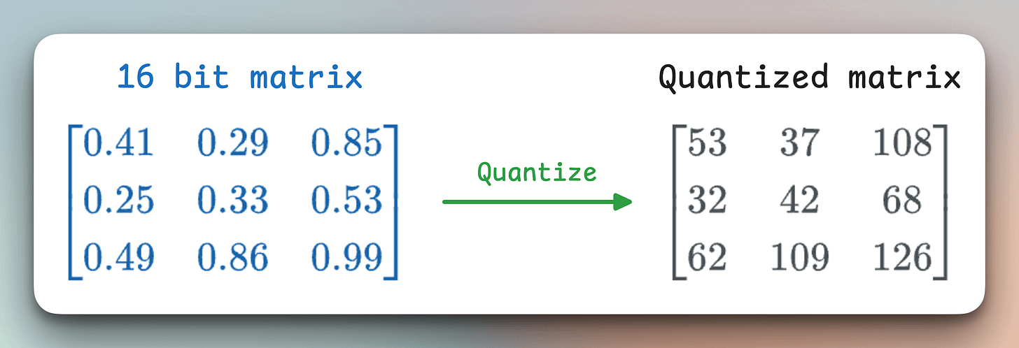
At 4-bit, the weight memory drops 4x. The 140GB model fits in 35GB, within the range of a single 40GB or 48GB card.

That said, if rounding were lossless in practice, one method would suffice, and the diagram below would have had one row:

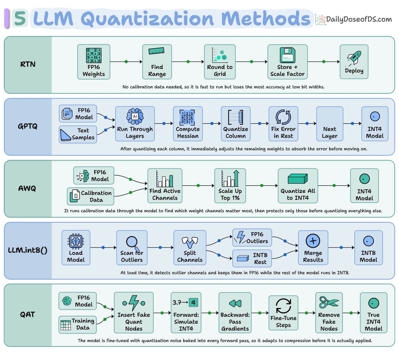
But it has five because weights and activations in large transformers are not uniformly important.

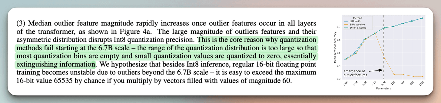
The LLM.int8() paper quantified this. Beyond roughly 6.7B parameters, every transformer layer develops a handful of hidden dimensions carrying values 20x to 100x larger than the rest.

These dimensions make up about 0.1% of the model’s features, but zeroing them out nearly destroys the model’s ability to predict text.

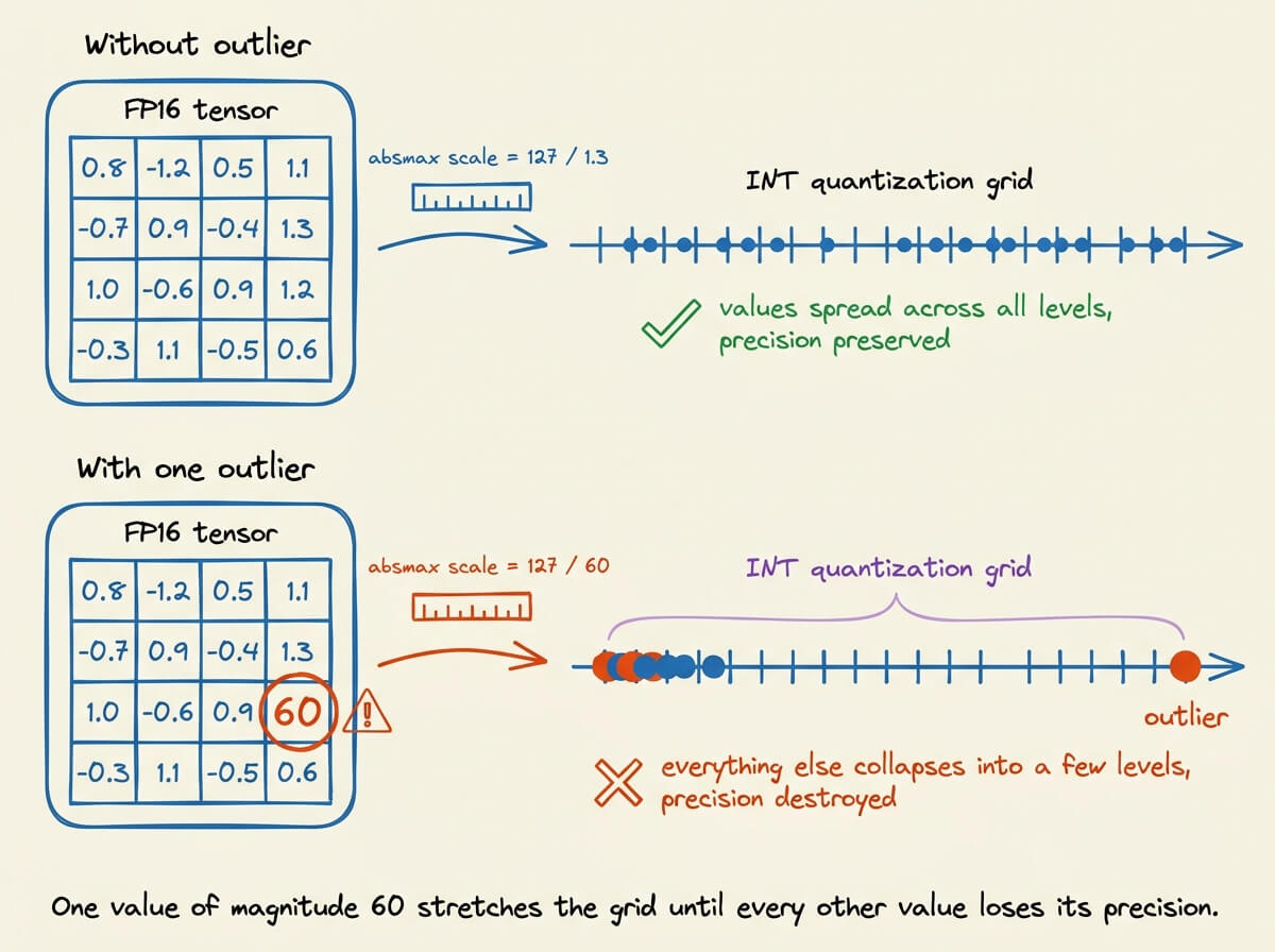
These outliers are also what break naive rounding. The quantization grid spans the range of the tensor, so a single activation of magnitude 60 among values near 1 inflates the scale factor and collapses the remaining values into a few levels, destroying their precision.

Each method in the visual shown earlier solves this saliency problem differently.

1) RTN (round to nearest) does not handle it at all. It applies the scale-and-round procedure directly with no calibration data, which makes it the cheapest baseline and the weakest at low bit widths, where accumulated rounding error is unrecoverable.

2) GPTQ corrects rounding damage as it happens. It quantizes the weights of a layer a few at a time, measures how much error the rounding just introduced, and nudges the not-yet-quantized weights to cancel out that error before moving on.

The adjustment is not uniform. GPTQ uses statistics from calibration data to work out which remaining weights can absorb the error with the least effect on the layer’s output, which is what separates it from blind rounding.

This runs fast enough to matter in practice. A 175B model quantizes to 4-bit in around four GPU hours. The known weakness is that fitting the calibration data this closely can tune the model to it, and the AWQ authors showed this hurts accuracy on inputs that look different from the calibration set.

3) AWQ protects the important weights before rounding instead of repairing damage afterward. It runs calibration samples through the model and watches which weights get multiplied by the largest incoming values, because a rounding error on those weights gets amplified the most in the layer’s output.

Only around 1% of weight channels turn out to matter this much. Rather than storing them at higher precision, AWQ multiplies them by a scaling factor before rounding, so they spread across more levels of the grid and lose less detail, and the math is rearranged so a matching inverse scale elsewhere keeps the layer’s output unchanged.

Every weight still ends up in plain INT4, with no special-case handling at inference time. AWQ also depends far less on which calibration samples were used than GPTQ does, which is a big part of why it became the standard choice in serving engines like vLLM.

4) LLM.int8() isolates the outliers instead of fighting them. When the model is loaded, it finds the dimensions carrying extreme values and splits every matrix multiplication into two:

• The outliers run in full FP16
• The other 99.9% of values run in INT8, and the two results are added back together.

Nothing needs to be computed ahead of time. That is why it is also available as the load_in_8bit flag in bitsandbytes.

The cost is speed. Splitting and merging every matrix multiplication is slower than running one optimized 4-bit kernel, so this path is common for local development and QLoRA fine-tuning, not for serving traffic at scale.

5) QAT modifies training rather than the quantization procedure. During a short fine-tuning run, every forward pass rounds the weights to INT4 before using them, so the model experiences the exact damage that quantization will cause, and its predictions are scored under that damage.

The weight updates still happen in full precision behind the scenes, since rounding itself cannot be trained through directly. Over the fine-tuning run, the weights drift toward values that keep the loss low even after rounding, so when the real quantization is applied at the end, there is almost nothing left to break.

Google produced its Gemma 3 QAT checkpoints with roughly 5,000 fine-tuning steps guided by the original model’s outputs, and the int4 versions hold close to full-precision quality at about 3x lower memory.

All five methods described above produce the same artifact, i.e., a model at a fraction of its trained precision.

They differ in where the outlier problem gets addressed, at rounding time, after rounding, before rounding, at inference, or during training itself.

To dive deeper, we have already written a full deep dive on Quantization, specifically, which covers several of these methods with their simplified mathematics.

Learn how Quantization optimizes LLMs to run them on tiny hardware here →

Good day!