Traditional data processing tools often fall short in big data projects – one in which the volume of data can be in the range of 100s of GBs.

This is because typical computing power is mostly limited to just a few gigabytes of RAM. As a result, loading a dataset at this massive scale for processing is impossible.

The above roadblock for analyzing large datasets is not just due to the unavailability of desired computing power but also due to the limitations of traditional data analysis tooling/libraries like NumPy, Pandas, Sklearn, etc.

This is because these tools are designed primarily for single-node processing. As a result, they struggle to seamlessly scale across multiple machines.

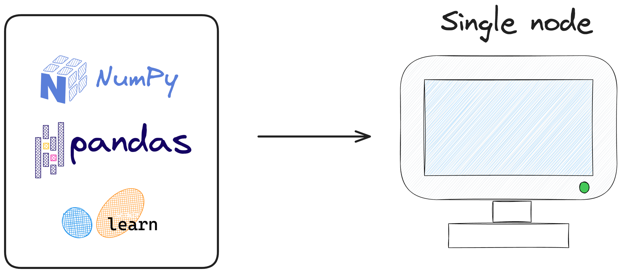
In other words, they operate under the assumption that the entire dataset can fit into the memory of a single machine.

However, this becomes impractical when dealing with datasets at scale.

Specifically talking about the enterprise space where data is mostly tabular, data scientists are left with very few options but to move to something like Spark, which is precisely used for such purposes.

Spark Basics

Before getting into any technical hands-on details about Spark, let’s understand what some details around:

• What is big data?
• What are distributed systems?
• What is Hadoop?
• What are the limitations of Hadoop?
• What is Spark and what is its utility in the context of big data projects?

What is big data?

Imagine we have a dataset that comfortably resides on a local computer, falling within the range of 0 to 32 gigabytes, or perhaps extending to 40-50 gigabytes, depending on the available RAM.

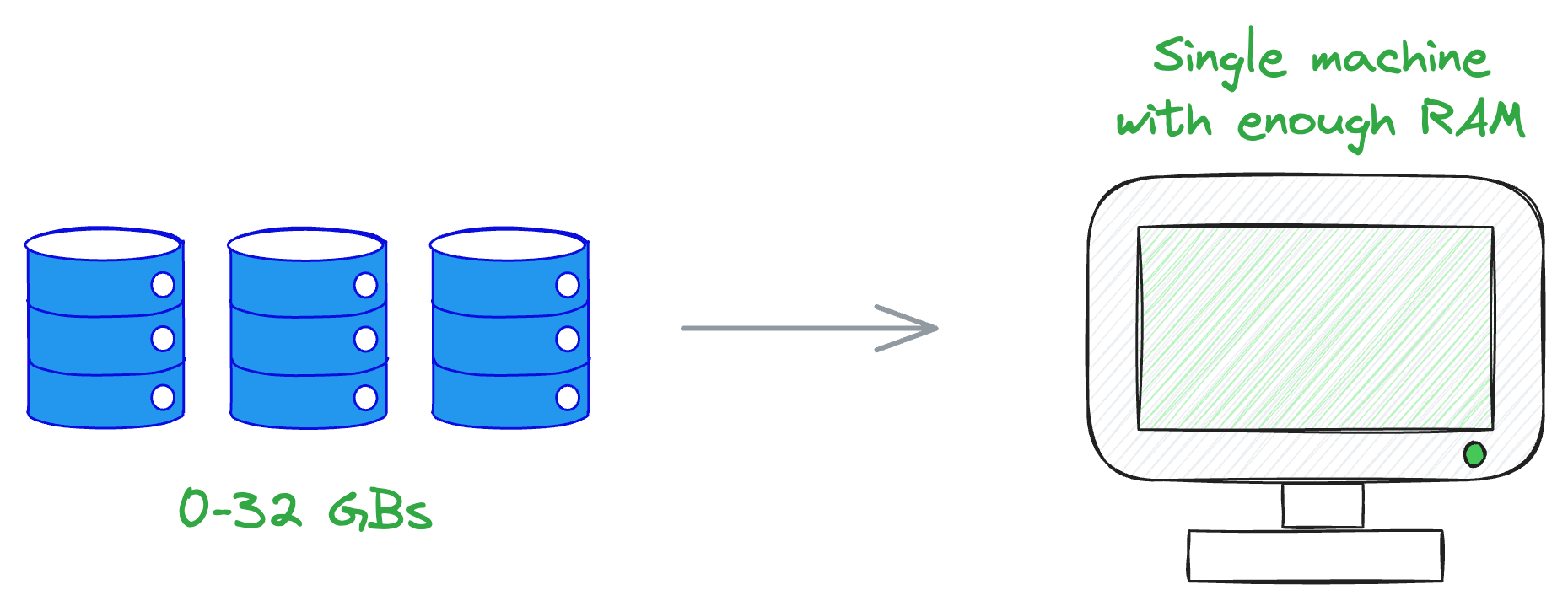
In this context, we're not typically dealing with big data.

Even if the dataset expands to, say, 30 to 60 gigabytes, it remains more feasible to acquire enough RAM to accommodate the entire dataset in memory.

RAM, or random access memory, is that swift-access, volatile storage used when, for instance, opening an Excel file—where all relevant data is stored temporarily for quick retrieval.

However, what if our dataset surpasses the limits of what can be held in memory?

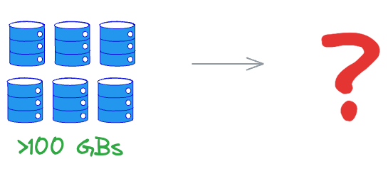
At this point, we face a decision point between the following two options:

SQL Database Approach

We could opt for a SQL database, shifting the storage from RAM to a hard drive.

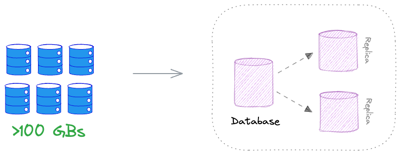
This approach allows us to manage larger datasets by leveraging the storage capacity of a hard drive, but it sacrifices the instantaneous and fast access provided by RAM.

Distributed Systems Solution

Alternatively, we can turn to a distributed system — a framework that disperses the data across multiple machines and computers.

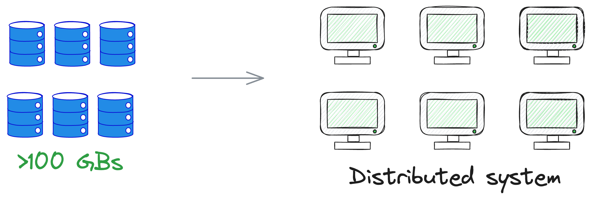
This becomes imperative when the dataset becomes too voluminous for a single machine or when the efficiency of centralized storage starts diminishing.

And here's where Spark becomes useful.

When we find ourselves considering Spark, we’ve reached a point where fitting all your data into RAM or a single machine is no longer practical.

Spark, with its distributed computing capabilities, lets us address the challenges posed by increasingly substantial datasets by offering a scalable and efficient solution for big data processing.

We shall come back to Spark shortly. Before that, let’s spend some time understanding the differences between local and distributed computing.

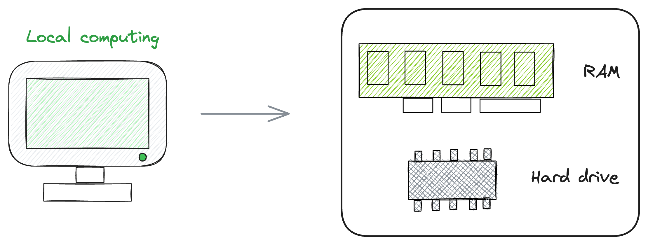
Local vs. distributed computing

While the names of these methodologies are pretty much sufficient to understand what they do, let’s understand what they are in case you are new to them.

In a local system, which you are likely to be familiar with and use regularly, operations are confined to a single machine — a solitary computer with a unified RAM and hard drive.

On the other hand, a distributed system, as depicted below, introduces a more intricate structure.

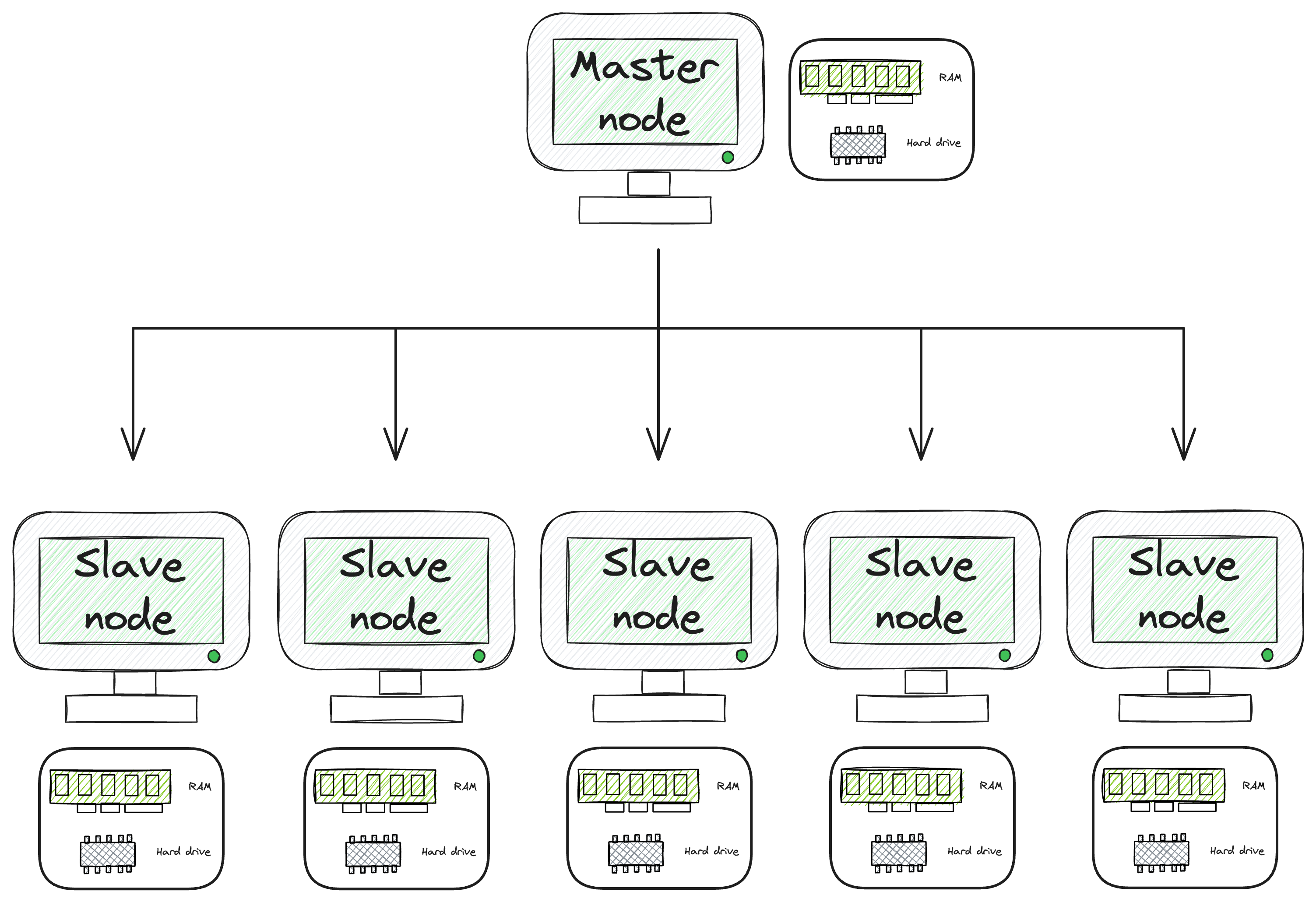
In a distributed system, there exists a primary computer, often referred to as the master node, alongside the distribution of both data and computational tasks to additional computers in the network.

The critical contrast lies in the capabilities of these systems, which we shall discuss next.

Local System Limitations and Distributed System Advantages

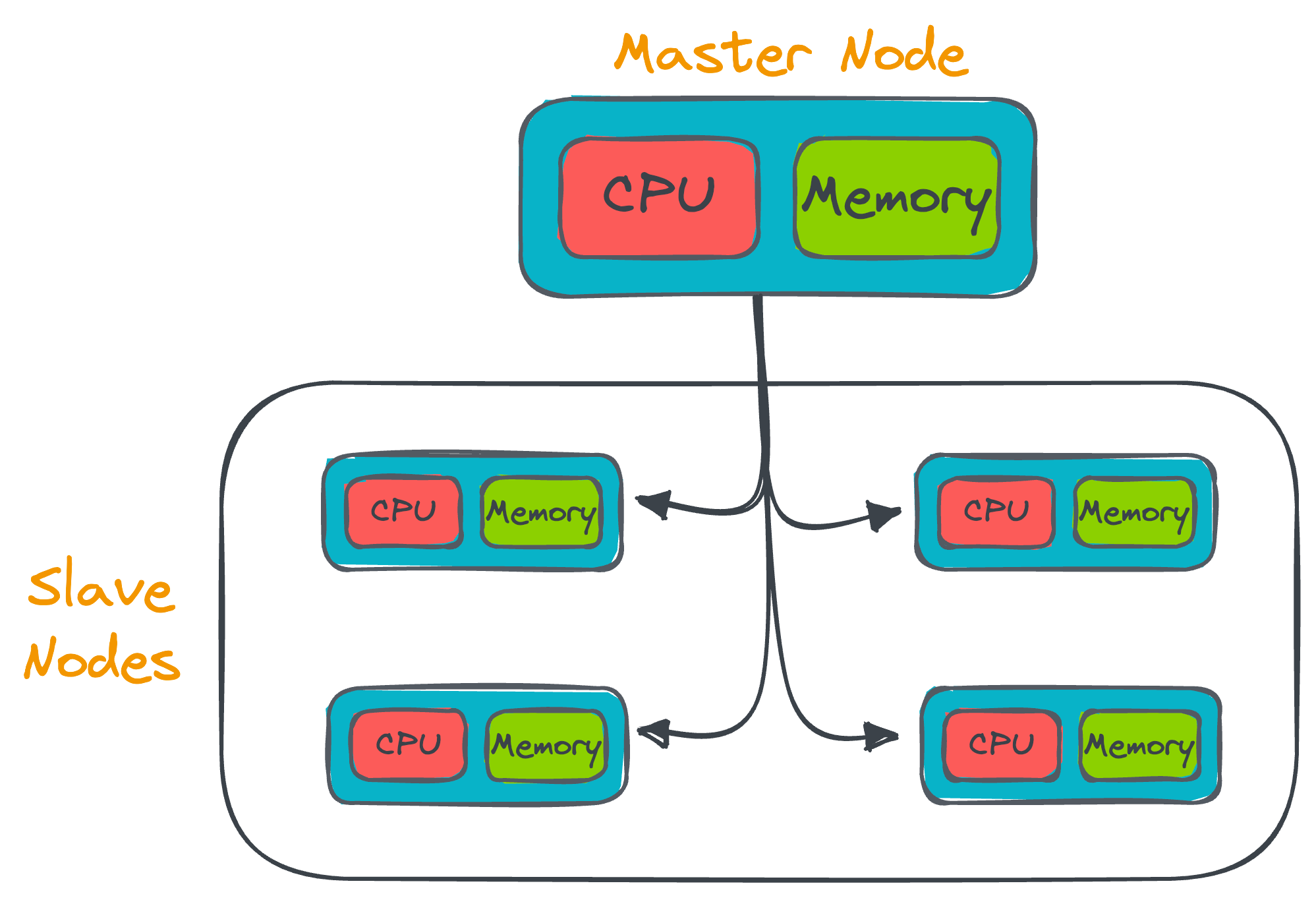
In local systems, the processing power and storage are confined to the resources available on the local machine, which is dictated by the number of cores and the capacity of the machine.

Distributed systems, however, leverage the combined power of multiple machines, allowing for a substantial increase in processing cores and capabilities compared to a robust local machine.

For instance, as illustrated in the diagram, a local machine might have, for instance, five cores.

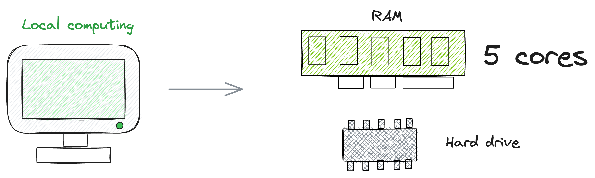
However, in a distributed system, the strategy involves aggregating less powerful machines, i.e., servers with lower specifications, and distributing both data and computations across this network.

This approach harnesses the inherent strength of distributed systems.

Scaling becomes a pivotal advantage of distributed systems over local systems.

More specifically, scaling a distributed system just means adding more machines to the network. In other words, one can significantly enhance processing power by simply adding more machines.

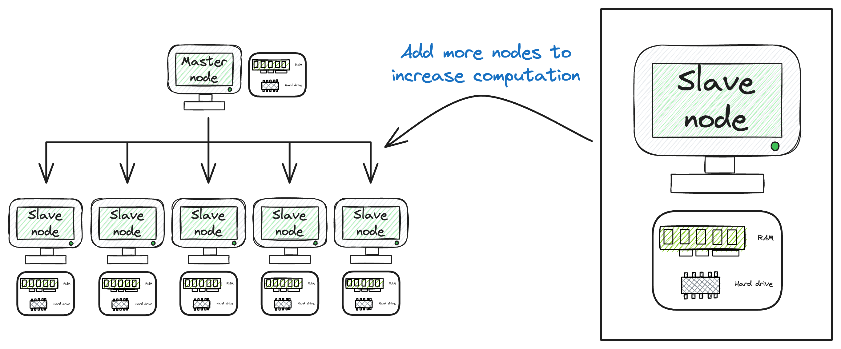
This technique proves more straightforward than attempting to scale up a single machine with higher CPU capacity.

What’s more, distributed systems are resilient to fault tolerance, a vital feature when dealing with substantial datasets.

As multiple machines work together, in the event of a machine failure, the distributed network can still remain active.

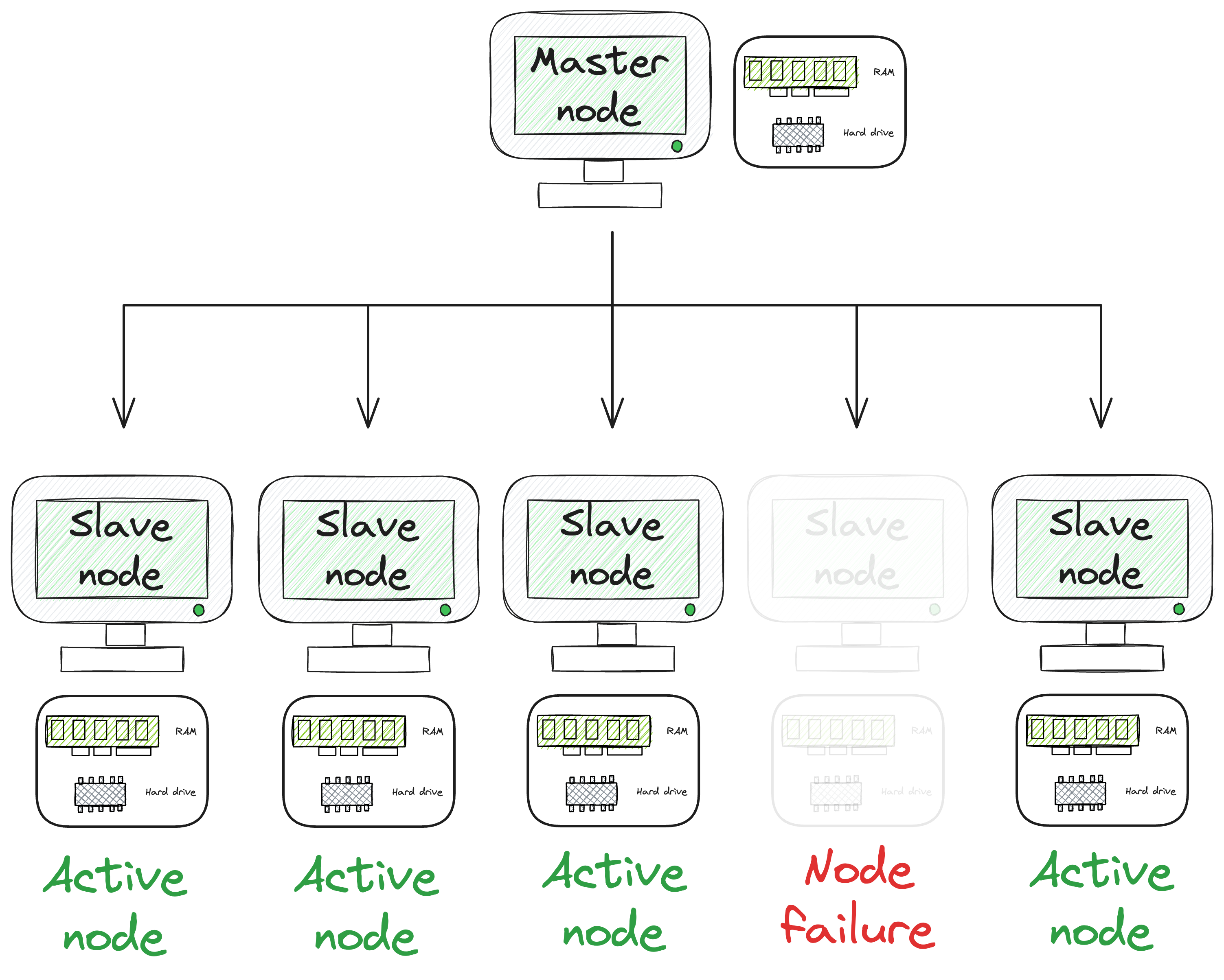
However, local machines are vulnerable to failures, where a crash could result in the loss of all ongoing calculations and data.

Back in the early 2000s, the development of Hadoop allowed us to effectively distribute these very large files across multiple machines and prevent these somewhat unpredictable failures.

And, of course, as we discussed above, traditional database systems and computing architectures were ill-equipped to handle datasets that were growing at an exponential rate.

What is Hadoop?

At its core, Hadoop is a distributed storage and processing framework designed to handle vast amounts of data across clusters (groups) of traditional hardware.

There’s no need to overcomplicate any technical details about what Hadoop is.

In a gist, it is a framework primarily meant for distributed storage and efficient data processing, particularly well-suited for big data projects.

There are two primary components in the Hadoop ecosystem.

#1) Hadoop Distributed File System

Hadoop Distributed File System (popularly known as HDFS) is used as a file storage system in Hadoop.

It is responsible for storing and keeping track of large data sets (both structured and unstructured data) across the various data nodes.

HDFS distributes data across a cluster of machines by breaking it into smaller blocks.

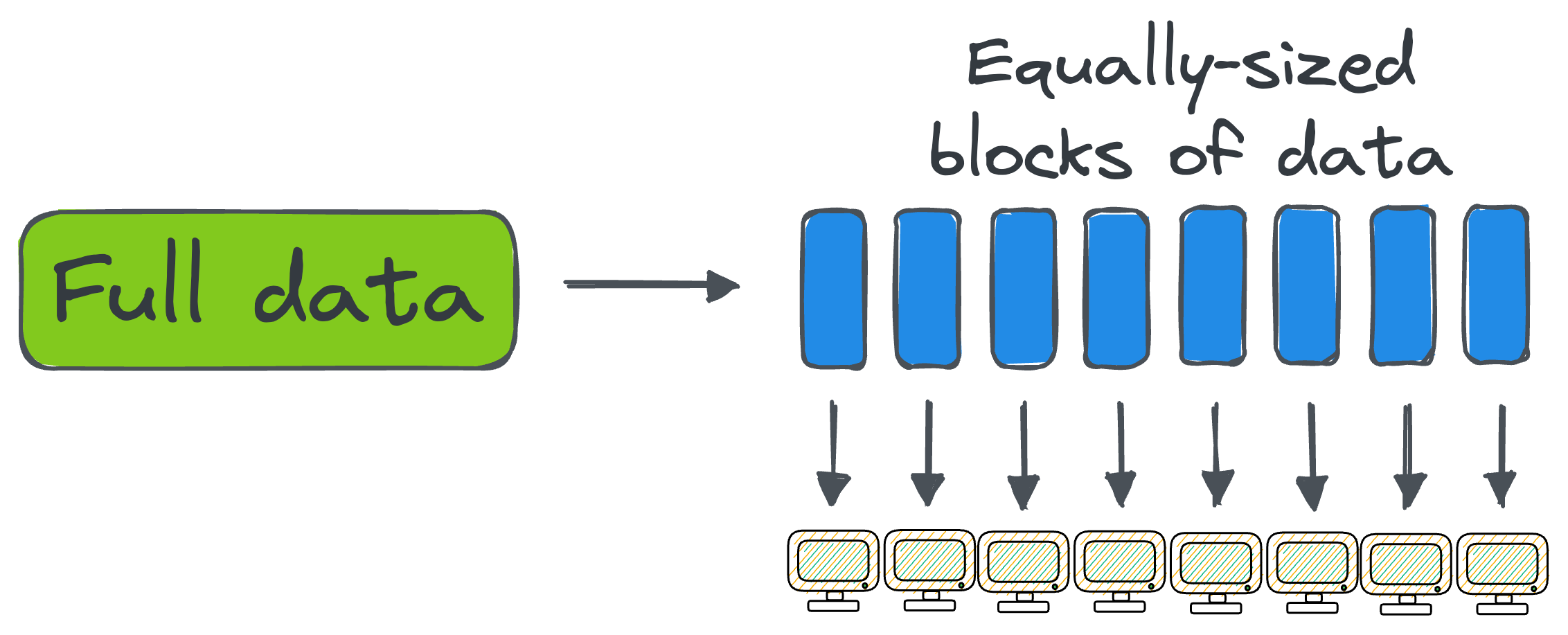
What’s more, HDFS ensures fault tolerance by replicating the same block across multiple nodes.

If one node goes down, it can use its data from another node so that processing does not stop at any point.

#2) Map Reduce

Map Reduce performs the operations on the distributed data.

It is a programming model and processing engine, that allows computations to be broken down into smaller tasks (this is called the Map step) and process them in parallel across the cluster.

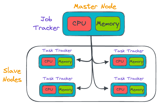
The master node (also called the job tracker) distributes the code/task that the slave node (also called the task tracker) must run.

The slave node is responsible for carrying out the received task on its end, updating the master node in case of any failures, and under successful execution, it must revert back to the master node with the generated results.

The results are then consolidated (this is called the Reduce step), thereby providing an efficient way to process vast amounts of data.

So, to summarize:

• Hadoop is a distributed computing framework that facilitates the processing of large datasets in clusters of computers.
• Hadoop Distributed File System (HDFS) is a fault-tolerant and scalable distributed file storage system used by Hadoop to handle massive amounts of data efficiently.
• Map Reduce is the processing engine within Hadoop that facilitates the computations across nodes and consolidates the results.

What is Spark?

Spark is now among the best technologies used to quickly and efficiently handle big datasets.

Simply put, Spark is an efficient alternative to the MapReduce step of Hadoop we discussed earlier.

So,. in a way, Spark is NOT an alternative to Hadoop, but rather an alternative to Hadoop MapReduce.

Thus, it must always be compared to Hadoop MapReduce and not entirely to Hadoop.

That said, unlike Hadoop, the utility of Spark is not just limited to HDFS. Instead, one can use Spark with many other file formats like:

• Apache Parquet
• HDFS
• JSON
• MongoDB
• AWS S3, and more.

Spark vs. MapReduce

As mentioned above, Spark is an efficient alternative to the MapReduce step of Hadoop, and it can be up to 100x faster than Hadoop MapReduce.

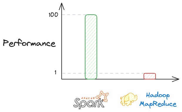
The significant speed difference between Spark and Hadoop MapReduce is primarily attributed to Spark's ability to perform in-memory processing.

Simply put, Hadoop MapReduce reads the data from the disk for each stage of processing and stores the data on the disk after every Map and Reduce step.

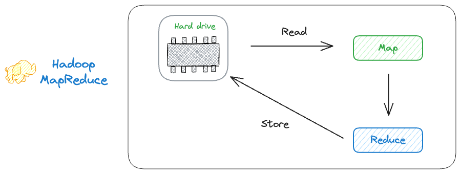
This leads to potential performance bottlenecks.

Spark, on the other hand, utilizes in-memory processing, thereby reducing the need to read and write to disk, which significantly speeds up iterative algorithms and iterative machine learning tasks.

If the memory utilization exceeds the available memory, Spark can leverage the disk to store the data on the disk.

The core idea is that if we don’t have enough memory, Spark will try to write the extra data to disk to prevent the process from crashing. This is called disk spill.

As discussed above, the reason why MapReduce is slow is because is intensively relies on reading and writing data to disk. Thus, while writing code in Spark, always attempt to avoid spill by processing less data per task. Otherwise, it can result in serious bottlenecks.

Here, we must note the fact that Spark is not a programming language. Instead, it is a distributed processing framework written in the Scala programming language.

But the utility of Spark is not just limited to Scala. Instead, Spark also has APIs for Python, Java and R.

The one that we will be learning in this deep dive is PySpark — the Python API of Spark for distributed computing.

The non-Scala API interacts with Spark, and provides four specialized packages for the following tasks:

1. Spark SQL: Enables integration of structured data using SQL queries (or equivalent DataFrame operations) with Spark.
2. Spark Streaming: Facilitates real-time processing and analytics on streaming data.
3. MLlib: Provides machine learning libraries and algorithms for data analysis and modeling.
4. GraphX: Offers a distributed graph processing framework for graph computation and analytics in Spark.

Spark RDDs

Spark Resilient Distributed Datasets (RDD) is the fundamental data structure of Spark.

For more clarity, like Pandas has a Pandas DataFrame data structure, Spark has RDDs.

Formally put, RDDs are the fundamental data structure in Apache Spark, representing an immutable, distributed collection of objects that can be processed in parallel.

A plus point of Spark RDDs is that, like HDFS, they provide fault tolerance, parallel processing, and the ability to work with large datasets across a cluster of machines.

Let’s discuss these properties in a bit more detail.

Key properties of Spark RDDs

1) Spark RDDs are Immutable

Once created, RDDs cannot be modified. Operations on RDDs generate new RDDs rather than modifying the existing ones. Why?

• Immutability is preferred because it ensures data consistency and simplifies the implementation of fault-tolerance mechanisms.
• With immutable RDDs, each transformation creates a new RDD with a clear lineage, representing a sequence of transformations applied to the original data.

• This lineage information allows Spark to recover lost data in the event of node failures by recomputing affected partitions based on the original data source.
• Immutability also enhances parallelism, as each partition of an RDD can be processed independently without concern for concurrent modifications, simplifying the management of distributed computations across a cluster of machines.

Summary: Immutability simplifies fault recovery and enables Spark to efficiently recover lost data by recomputing it from the original source.

2) Spark RDDs are Distributed

RDDs are distributed across multiple nodes in a Spark cluster.

Each partition of an RDD is processed independently on a different node, enabling parallelism.

3) Spark RDDs are Fault-Tolerant

RDDs are resilient to node failures. If a partition of an RDD is lost due to a node failure, Spark can recompute that partition from the original data using the lineage information (the sequence of transformations that led to the creation of the RDD).

4) Spark RDDs provide Lazy Evaluation

Spark employs lazy evaluation, meaning transformations on RDDs are not executed immediately. Transformations are only executed when an action is called, allowing for optimization of the entire sequence of transformations.

Operations on Spark RDDs

We can carry out two types of operations on Spark RDDs.

1. Transformations
2. Actions

Let’s understand them one by one.

1) Spark Transformations

A Transformation in Spark refers to the process of creating new RDDs from the existing ones.

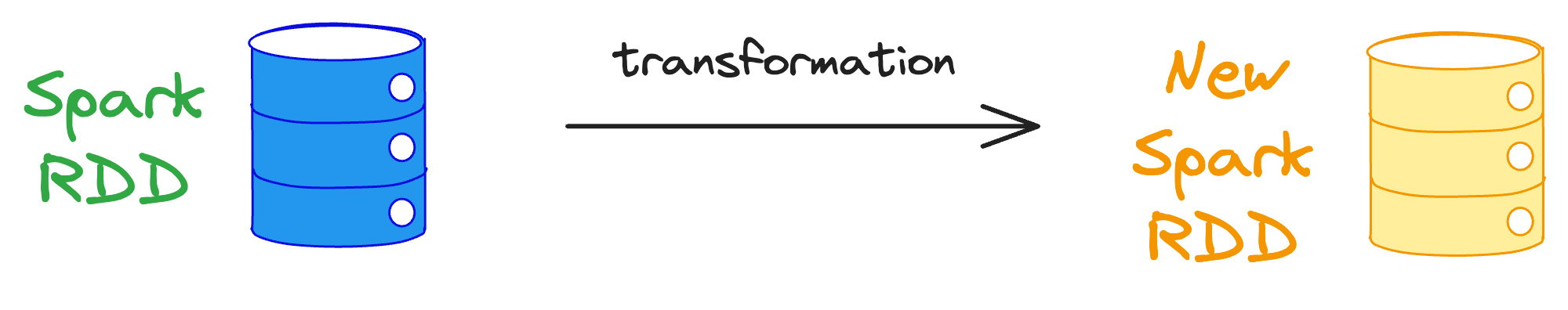
It involves following the user-defined functions to the elements of an RDD to generate a desired output.

The primary purpose of transformations is to modify the current dataset into the desired dataset, effectively transforming the data based on specified computations.

A key point to note here is that transformations do not alter the original RDD. Instead, they generate new RDDs as a result of the applied operations because of the immutability property of Spark RDDs.

Another critical aspect of Spark transformations is that they follow lazy evaluation.

Lazy evaluation implies that the execution of transformations does not produce immediate results until we invoke some output to memory.

Instead, the computations are deferred until an action is triggered. This makes sense because it lets Spark optimize the execution workflow and resource utilization.

In other words, laziness in evaluating transformations allows Spark to build a logical execution plan, represented by the RDD lineage, without immediately executing each step.

In fact, we will also see this shortly when we experiment with PySpark DataFrames. When we will write a method call, we won’t get any output immediately until we call an action.

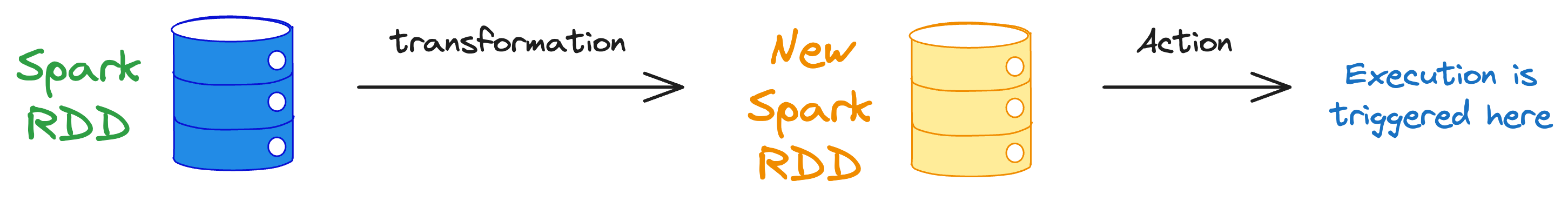
2) Spark Actions

Actions in Spark are operations that actually trigger the execution of computations and transformations on RDDs, providing a mechanism to obtain results and send them back to storage or the program.

Unlike transformations, which are lazily evaluated, actions force the evaluation of the entire lineage and execution of the logical execution plan.

There are three types of actions:

• When we wish to view/print the data.
• When we want to write the data to a storage source.
• When we want to bring data to, say, Python lists/arrays etc.

Another key point to note here is that while transformations return new RDDs, actions yield results in other data types.

In other words, Spark actions provide non-RDD values to the RDD operations, allowing users to obtain concrete and readable outcomes from the distributed computations.

Let’s dive into the programming stuff now.

Setting up PySpark

In this section, we shall learn about how to set up PySpark to use it in a Jupyter Notebook.

Please feel free to skip this part if you already have PySpark set up on your local computer.

But one thing to note here is that we don’t run Spark on one machine. Instead, in typical big data settings, Spark runs on a cluster of computers, which are all always Linux-based.

Of course, there are ways to do that and mimic some sort of a “real-world” setting of clusters.

But I intend to make this deep dive as practical and realistic as possible.

Thus, when it comes to setting up Spark, it won't be really about setting it up on your local machine. Instead, it will be about connecting your machine to an online Linux-based server where we can use Spark.

Thus, the Linux-based servers that we shall be using in this deep dive will be from Databricks. They provide a free community version,are which you can utilize in this article to learn about PySpark.

Please note that the syntax of Spark will remain unchanged irrespective of where your clusters are set up. This is because clusters mainly provide computational power, which is precisely what we desire in big data settings.

That said, if you still want to learn the syntax on your local computer, you are free to do that too. Follow this guide to install PySpark:

• MacOS: https://sparkbyexamples.com/pyspark/how-to-install-pyspark-on-mac/.
• Windows: https://sparkbyexamples.com/pyspark/how-to-install-and-run-pyspark-on-windows/.

Setting up Databricks

To begin set up, head over to the Databricks setup page and create an account.

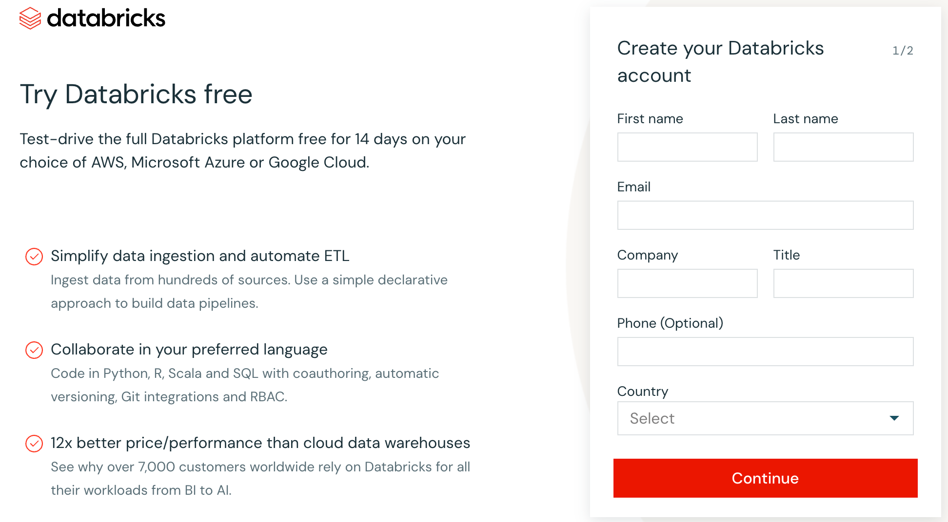
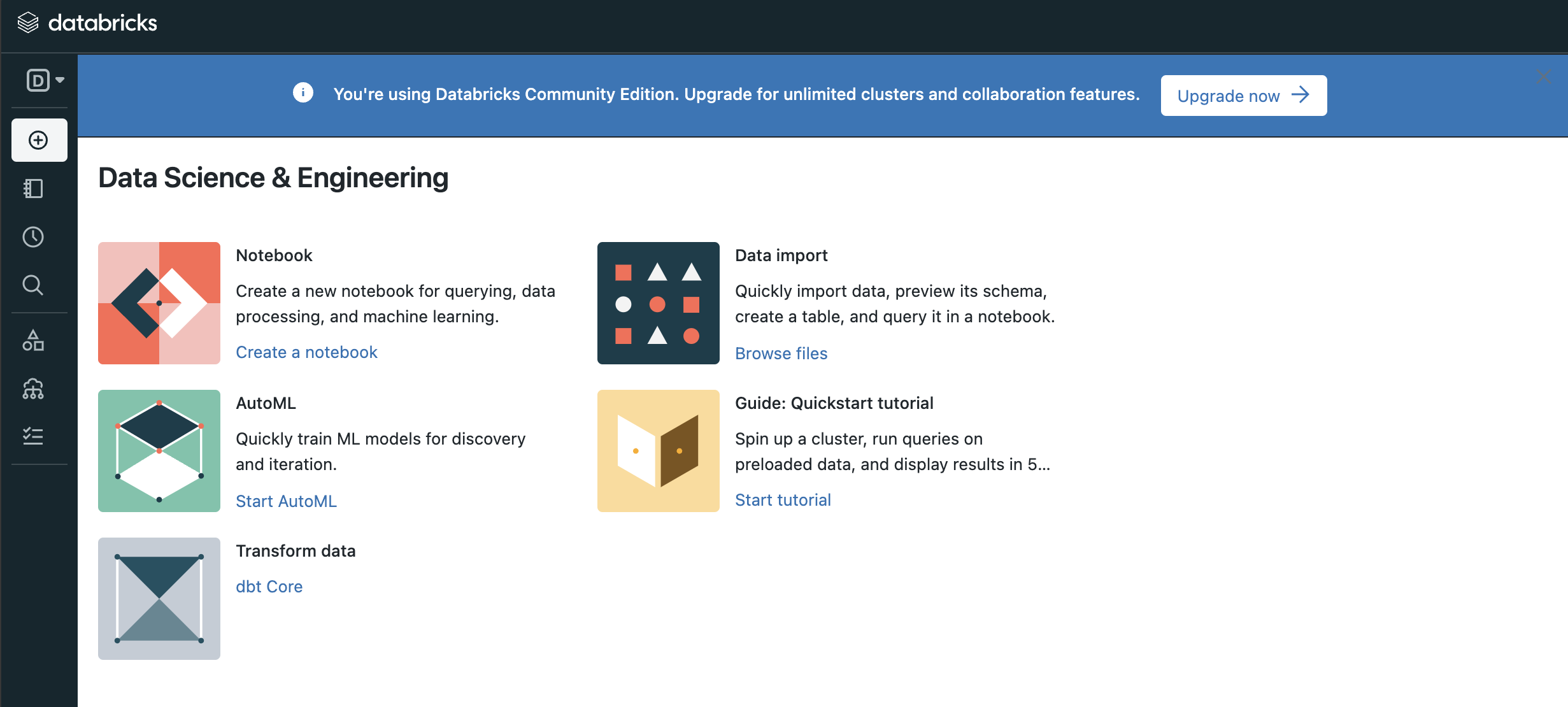
After filling up the details above, Databricks will take you to the following page:

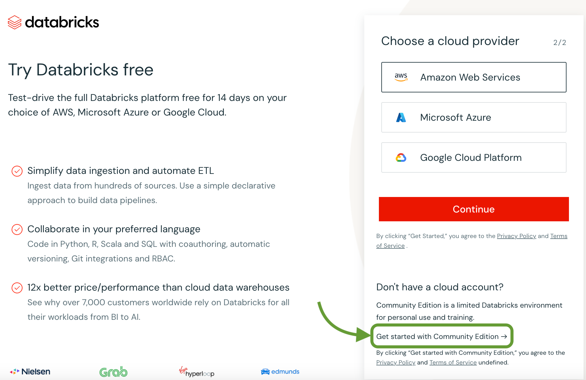
Select the community edition above.

Once you select that, Databricks will ask you to verify your email.

During verification, it will ask you to create a password. Complete that step to set up the Databricks community edition account.

This will provide us with a cluster of 15 GBs, which, admittedly, is not that big, but it’s okay as we are just learning right now.

Also, as you would transition towards large projects, your employer will ensure that you have large enough clusters, and the syntax will remain the same anyway.

Setup Databricks cluster

As we discussed above, we must set up a cluster to mimic and leverage the distributed functionalities of Spark.

Simply put, Spark’s power lies in its ability to distribute and parallelize data processing tasks across multiple nodes within a cluster.

When dealing with vast amounts of data that surpass the capacity of a single machine, a clustered environment becomes imperative.

And to recall, a cluster is a network of interconnected machines, or nodes, working collaboratively to process and analyze large datasets efficiently.

By distributing the workload across the nodes within a cluster, Spark can harness the combined computational power and memory resources of these machines.

This parallel processing capability not only enhances performance but also enables Spark to handle massive datasets that would be impractical to process on a standalone machine.

This step is demonstrated in the video below:

Select the Databricks runtime version as the preselected one.

Done!

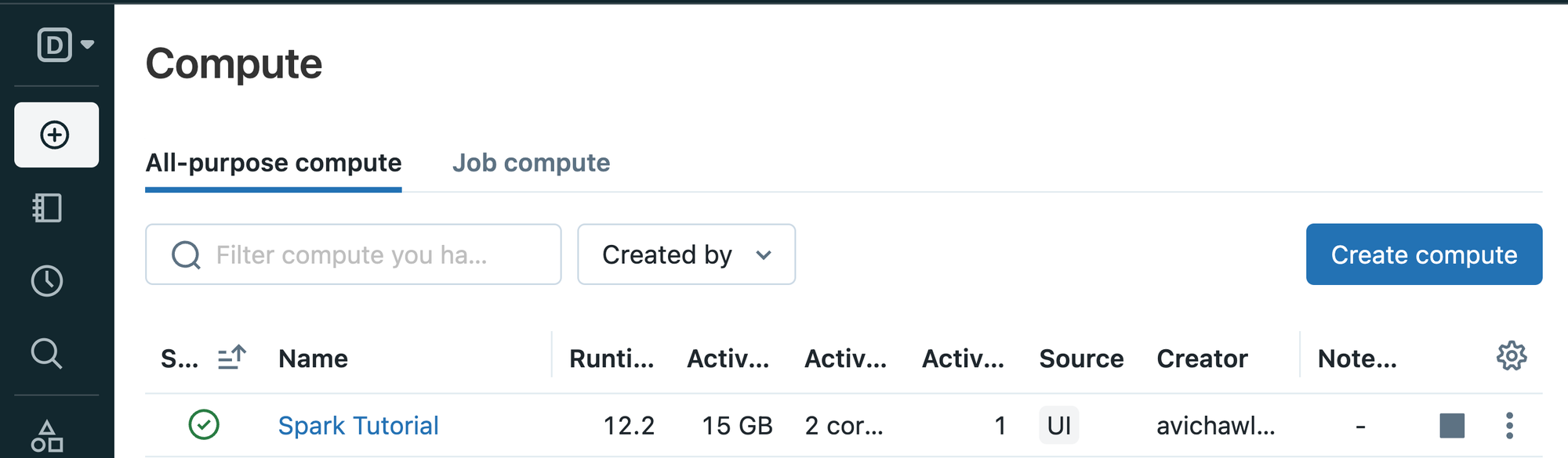
Next, we will see an active cluster in the Databricks dashboard. As depicted below, it has 15 GB of memory.

Setup Databricks notebook

The final step in this Databricks setup is to create a new Jupyter notebook, which we shall connect to the above cluster to leverage distributed computing.

In other words, the Jupyter Notebook becomes the interface through which we harness the computational capabilities of the clustered environment powered by Databricks.

The steps are demonstrated in the video below:

The above video also shows that we can use Spark with different languages like SQL, Scala, and R. We also discussed this earlier in the article.

The notebook also shows the cluster to which our Jupyter Notebook is connected to.

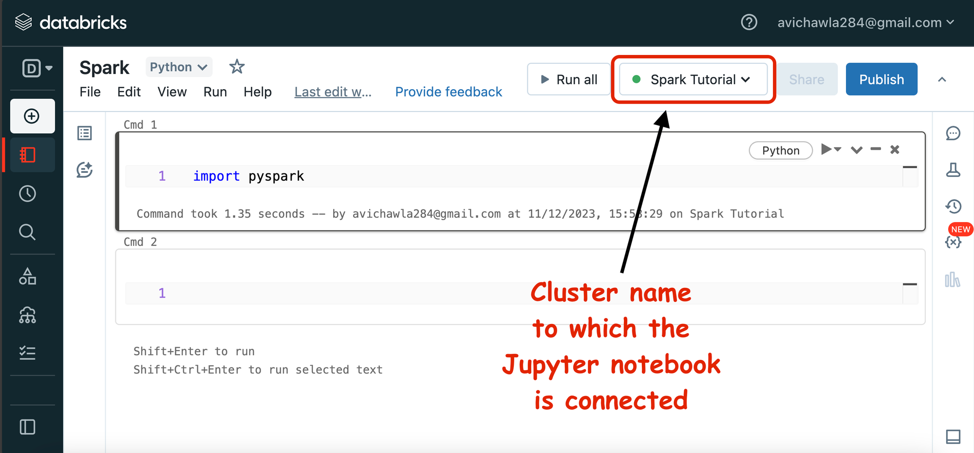
Once the notebook is set up, run import pyspark to test if it is working fine or not.

With this, we are done with the Databricks notebook set up in just three simple steps:

1. Create a Databricks community edition account.
2. Launch a cluster.
3. Launch a Jupyter Notebook and connect it to the cluster.

Upload data to Databricks

Of course, using Spark only makes sense when we have some data to work with.

For this exploratory tutorial, we shall be considering the following employee dataset:

The steps to upload the dataset are shown in the video below:

In the above video, after uploading the dataset, we select Create table with UI. This step allows us to specify the header for our uploaded file, the delimiter, etc.

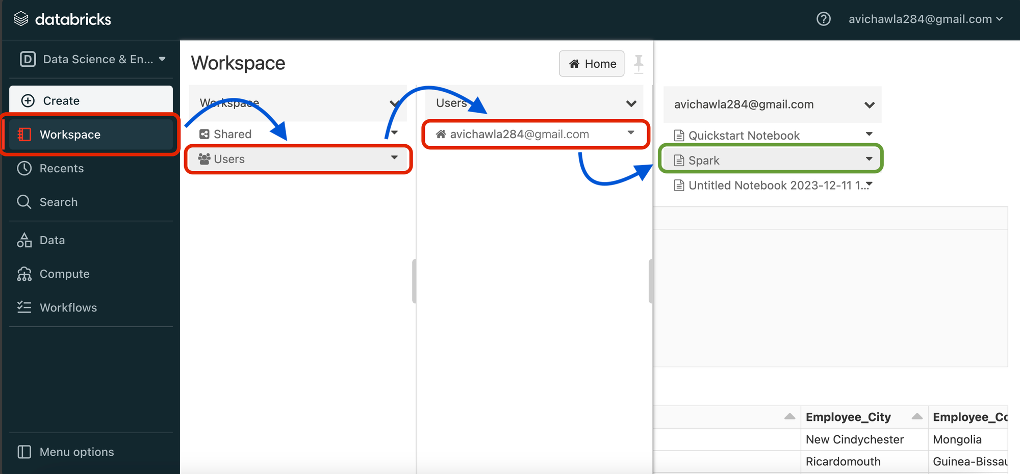
Once done, we head back to the Spark notebook as follows:

On a side note, although in this tutorial, we are uploading the dataset ourselves using a CSV file, this is not always necessary when using Spark.

In fact, Spark is pretty versatile when it comes to connecting to various data sources.

If you end up using Spark in any of the projects, then typically, you would end up loading datasets directly from the database because that’s how the engineers usually set up the infrastructure.

In practical scenarios, the workflow often involves the creation of datasets through SQL queries that aggregate and transform information collected from diverse sources.

These sources may include databases, data warehouses, data lakes, or external APIs. Engineers design SQL queries to extract, filter, and aggregate relevant data, forming a dataset that meets the analytical requirements of the project.

Once the dataset is constructed using SQL queries, Spark comes into play for further analysis.

Connecting Spark directly to the database eliminates the need for manual data uploads or intermediary storage steps, streamlining the data processing pipeline.

This approach not only enhances efficiency but also ensures that the analysis is performed on the most up-to-date and comprehensive dataset.

Hands-on PySpark

Now, let’s get to the fun part of learning the PySpark syntax.

PySpark DataFrames

The focus of this section is to deep dive into PySpark DataFrames.

If you are familiar with Pandas, you may already know that DataFrames refer to tabular data structures – one with some rows and columns.

PySpark DataFrames are distributed in-memory tables with named columns and schemas, where each column has a specific data type.

Spark DataFrame vs Pandas DataFrame

The notion of a Spark DataFrame is pretty similar to a Pandas DataFrame – both are meant for tabular datasets, but there are some notable differences that you must always remember:

• Spark DataFrames are immutable, but Pandas DataFrames are not.
  • As discussed earlier, Spark relies on RDDs, which are the fundamental data structure in Spark. By its very nature, they represent an immutable, distributed collection of objects that can be processed in parallel.
  • Thus, after creating a Spark DataFrame we can never change it.
  • So after executing any transformation, Spark returns a new DataFrame.
• Spark DataFrames are distributed, but Pandas DataFrames are not.
  • Pandas code always runs on a single machine, that too on a single core of a CPU.
  • However, Spark code can be executed in a distributed way. In fact, that is the sole purpose of Spark – distributed computing. This makes Spark DataFrames distributed in nature.
• Spark follows lazy execution but Pandas follows eager execution.
  • Lazy evaluation is a clever execution strategy wherein the evaluation of some code is delayed until its value is needed.
  • As discussed earlier, Spark provides two types of operations:
    • Transformations: These operations transform a Spark DataFrame into a new DataFrame.
    • Actions: Actions are any other operations that do not return a Spark DataFrame. Their prime utility is for operations like displaying a DataFrame on the screen, writing it to storage, or triggering an intentional computation on a DataFrame and returning the result.
  • In Spark, transformations are computed lazily and their execution is delayed until an action is invoked.
  • In Pandas, however, all operations are eagerly evaluated.

#0) Spark Session

To use Spark’s capabilities and Spark DataFrames, we must first create a Spark session.

You can think of Spark session as an entry point to the functionality provided by Spark. By declaring a Spark session, we get an interface through which we can interact with Spark’s distributed data processing capabilities.

In other words, creating a Spark session connects an application with the Spark cluster. Thus, for one Spark application, there can only be one Spark Session.

This invocation encapsulates the configuration settings and resources needed for Spark applications to run efficiently.

Thus, when creating a Spark session, users can define various parameters, such as application name, cluster configuration, and resource allocation, to tailor the session to specific requirements.

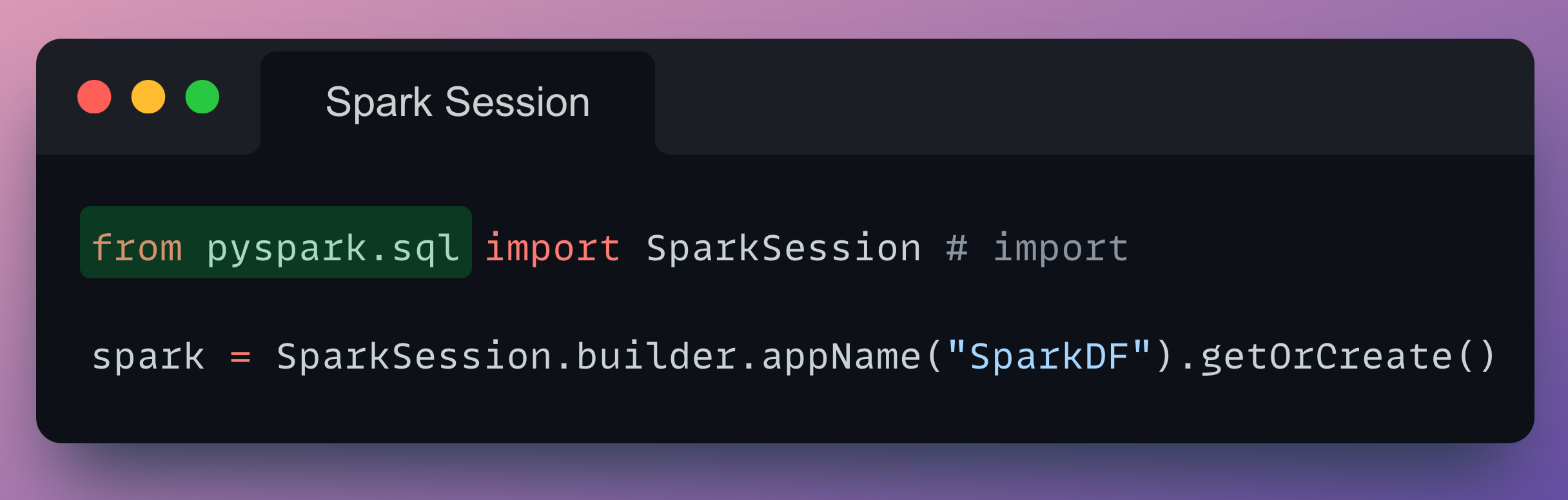
We declare a Spark Session as follows:

Let's break down each part of the code:

• SparkSession.builder:
  • The builder method is used to create a SparkSession.Builder instance.
  • The builder is a configuration interface for Spark sessions, allowing users to set various options and parameters before finally creating the Spark session.
• appName("SparkDF"):
  • The appName method sets a name for the Spark application.
  • In this case, the application name is set to SparkDF. This name is often used in the Spark UI and logs, providing a human-readable identifier for the application, which is especially useful when many users are interacting with a cluster.
• getOrCreate():
  • The getOrCreate method attempts to retrieve an existing Spark session or creates a new one if none exists.
  • This is particularly useful when working in interactive environments like Jupyter notebooks, where multiple sessions might be created.
  • The existing Spark session is retrieved if available, ensuring that resources are not wasted by creating multiple Spark sessions.

Once we run the above command, it is quite normal to take a minute or so sometimes as Spark tries to gather the specified resources.

After execution, we get a SparkSession object.

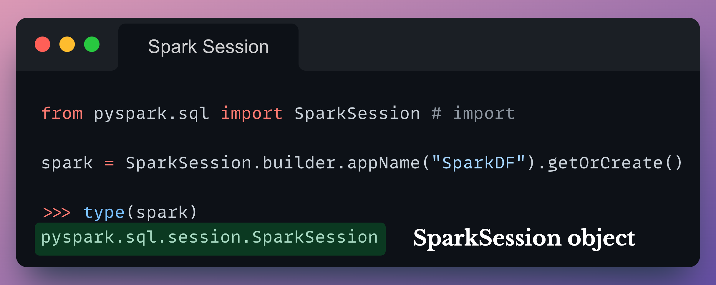
We can use this object to interact with the Spark cluster and perform various data processing tasks.

In other words, the SparkSession serves as our entry point to Spark functionalities.

We can use this object for:

• Creating DataFrames
• Executing Spark SQL Queries
• Configuring Spark Properties
• Accessing Spark's Built-in Functions
• Managing Spark Jobs
• and many many more tasks.

Here, if we print the spark object created above, we get the following output:

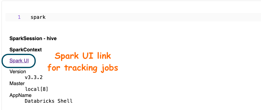
Opening the above link, we get to the following page:

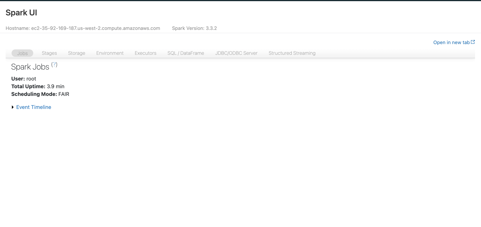
We will look at Spark UI ahead in the article, but this is the interface that provides us with in-depth information about the execution of our Spark jobs, transformations, actions, and more.

#1) Row objects

In PySpark, a DataFrame is essentially a distributed collection of rows organized under named columns.

Each row in a DataFrame can be conceptualized as a sequence of row objects.

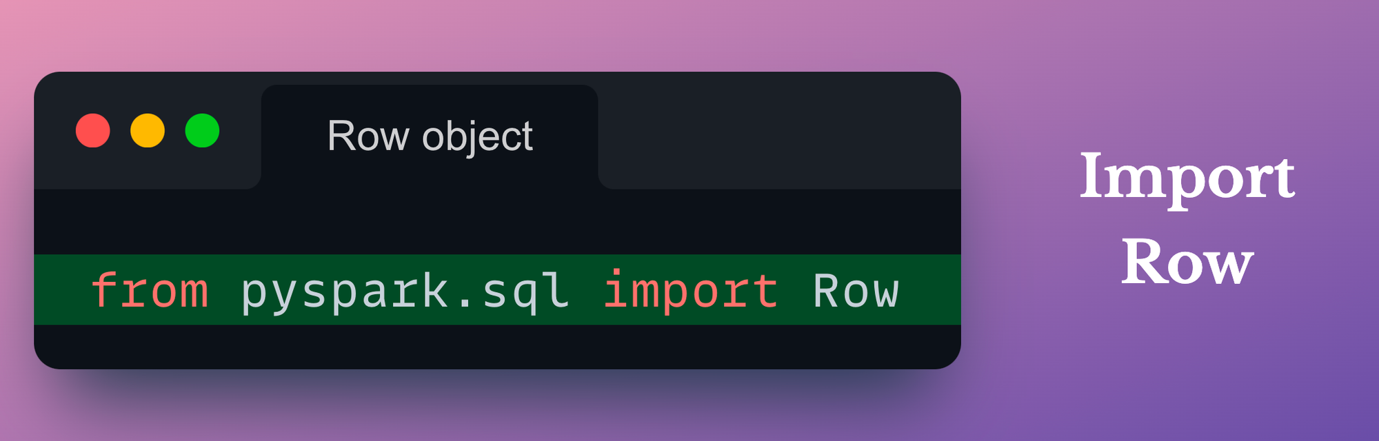
Import Row class

In PySpark, these row objects are instances of the generic Row class, which is imported as follows:

On a side note, the pyspark.sql package implements a comprehensive set of tools and functionalities for structured data processing using PySpark.

It serves as the SQL interface for working with distributed data in a tabular form, providing a high-level API for creating, querying, and manipulating DataFrames.

In fact, most of the DataFrame-related functionalities you would use in PySpark will be found in the pyspark.sql package.

Even SparkSession is implemented in the pyspark.sql package:

Now, coming back to the Row class, we import it as follows:

The Row class in PySpark serves as a blueprint for creating row objects within a DataFrame.

When we create a DataFrame, each row is represented as an instance of this generic Row object.

Define Row objects

Thus, we can instantiate standalone row objects by specified named arguments corresponding to the column names in the DataFrame.

This is demonstrated below:

As depicted above, once a row object is created, its elements can be accessed either by their names (column names) or by using index-based access.

Missing arguments

Here, we must note that when declaring Row objects of some standard schema, we are not allowed to omit a named argument:

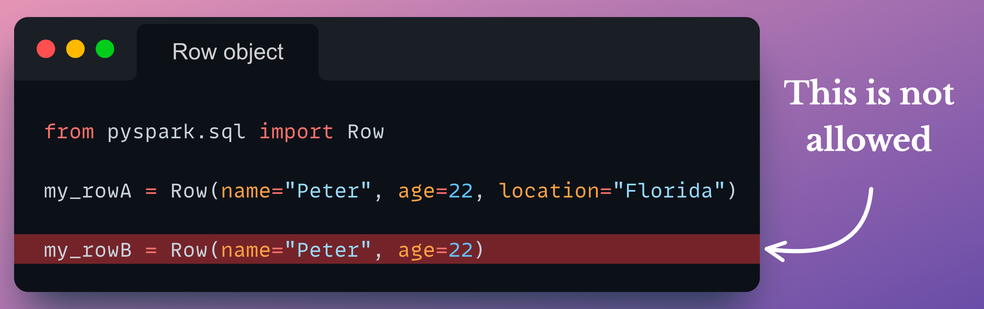
Of course, the my_rowB object can exist as a standalone Row object, but the point is that my_rowB and my_rowA cannot be combined into the same DataFrame at a later point. We will also verify this shortly.

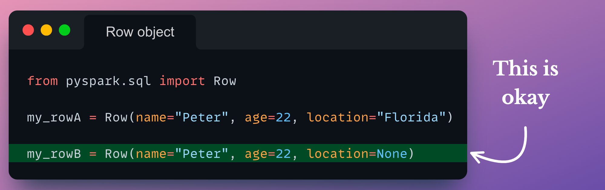
Thus, if you are creating Row objects that belong to a standard schema, and some of its named arguments are None, they MUST be explicitly set to None in such instances:

Standard schema for Row object

At times, creating many Row objects by specifying the named arguments can be tedious: