Implementing LLaMA 4 from Scratch

Introduction

In recent months, LLaMA 4 has sparked plenty of conversation, not just because of its performance, but because of how it achieves that performance.

Unlike previous generations, LLaMA 4 doesn’t rely solely on the classic Transformer architecture. Instead, it uses a Mixture-of-Experts (MoE) approach, activating only a small subset of expert subnetworks per token.

This allows it to scale to hundreds of billions of parameters while keeping inference efficient and cost-effective.

But how does that actually work under the hood?

In this article, we’ll answer that by building an MoE-based Transformer from scratch. It will be a miniature, interpretable version of LLaMA 4, using nothing but Python and PyTorch.

By doing so, we’ll demystify the architecture powering modern LLMs like LLaMA 4 and Mixtral, and give you hands-on insight into how experts, routers, and sparse activation work in practice.

We'll walk through every stage of implementation:

• Character-level tokenization,
• Multi-head self-attention with rotary positional embeddings (RoPE),
• Sparse routing with multiple expert MLPs,
• RMSNorm, residuals, and causal masking,
• And finally, training and generation.

Along the way, we’ll discuss why MoE matters, how it compares to standard feed-forward networks in Transformers, and what tradeoffs it introduces.

The goal is to help you understand both the theory and mechanics of MoE Transformers, not by reading another paper or GitHub README, but by building one line by line.

Let’s begin.

Why Mixture-of-Experts for LLMs?

Large Language Models (LLMs) have grown massively in size, reaching tens or even hundreds of billions of parameters. One recent innovation to make these models more efficient is the Mixture-of-Experts (MoE) architecture.

Instead of every part of the model being active for every input, MoE networks activate only a subset of “expert” sub-networks for each token.

This means only a fraction of the model’s parameters are used for each forward pass, reducing computation cost while preserving performance.

In other words, MoE lets us scale model capacity without a proportional increase in compute requirements.

To put it in perspective, Meta’s LLaMA 4 (the latest in the LLaMA series of LLMs) adopts an MoE architecture.

For example, LLaMA 4 Maverick uses 128 experts but activates just a few per token, achieving GPT-4-level performance at roughly half the inference cost.

MoE is a big reason why LLaMA 4 can be so large yet efficient – a sign of how important this idea is in current AI research.

How do MoEs work?

Mixture of Experts (MoE) is a popular architecture that uses different "experts" to improve Transformer models.

The visual below explains how they differ from Transformers.

Let's dive in to learn more about MoE!

Transformer and MoE differ in the decoder block:

• Transformer uses a feed-forward network.
• MoE uses experts, which are feed-forward networks but smaller compared to that in Transformer.

During inference, a subset of experts are selected. This makes inference faster in MoE.

Also, since the network has multiple decoder layers:

• the text passes through different experts across layers.
• the chosen experts also differ between tokens.

But how does the model decide which experts should be ideal?

The router does that.

The router is like a multi-class classifier that produces softmax scores over experts. Based on the scores, we select the top K experts.

The router is trained with the network and it learns to select the best experts.

But it isn't straightforward.

There are challenges.

Challenge 1) Notice this pattern at the start of training:

• The model selects "Expert 2" (randomly since all experts are similar).
• The selected expert gets a bit better.
• It may get selected again since it’s the best.
• This expert learns more.
• The same expert can get selected again since it’s the best.
• It learns even more.
• And so on!

Essentially, this way, many experts go under-trained!

We solve this in two steps:

• Add noise to the feed-forward output of the router so that other experts can get higher logits.
• Set all but top K logits to -infinity. After softmax, these scores become zero.

This way, other experts also get the opportunity to train.

Challenge 2) Some experts may get exposed to more tokens than others, leading to under-trained experts.

We prevent this by limiting the number of tokens an expert can process.

If an expert reaches the limit, the input token is passed to the next best expert instead.

MoEs have more parameters to load. However, a fraction of them are activated since we only select some experts.

This leads to faster inference. Mixtral 8x7B by MistralAI is one famous LLM that is based on MoE.

Most recently, Llama 4 also adhered to the MoE architecture, which is exactly what we are mimicking today!

Analogy #1 to understand MoEs

Training one giant neural network to “know everything” is hard.

Imagine instead you have a team of specialists, each expert at a certain type of task, plus a manager who assigns work to the best-suited specialist.

For example, if you’re running a company, you might hire an electrician, a plumber, a painter, each excels at different jobs; and a manager who decides which specialist should handle a given problem.

That’s essentially how an MoE model works! Instead of one monolithic network handling all inputs, an MoE layer contains multiple expert subnetworks (usually simple feed-forward networks), and a small router network that chooses which expert(s) should process each input token.

As shown in the figure above, a router (gate) receives each token’s representation and decides which expert networks to activate for that token.

In this sketch, the router chooses among four expert MLPs. Only the selected expert(s) perform computations for the token, and their outputs are combined.

This sparse activation allows the model to scale up the number of experts without increasing computation for each token.

Concretely, the router produces a set of scores or weights for the experts based on the token’s features.

It then selects the top-scoring expert(s) (say the best 2 or 3) and sends the token’s data to those experts.

The chosen experts each output a transformed vector, and the router uses its scores to weight and combine those expert outputs back into a single output vector for the token.

All other experts remain inactive for that token, saving compute. Different tokens in the same batch can go to different experts depending on the content. This way, an MoE layer dynamically allocates specialized processing for each token.

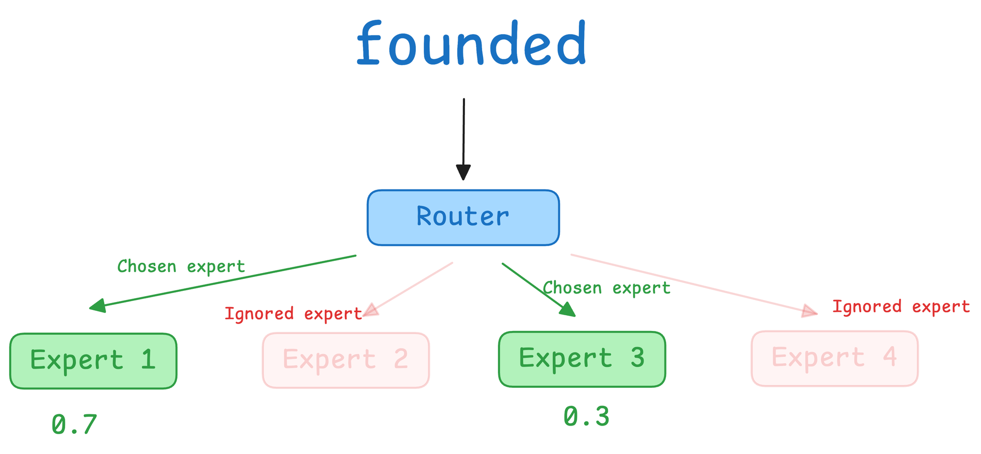
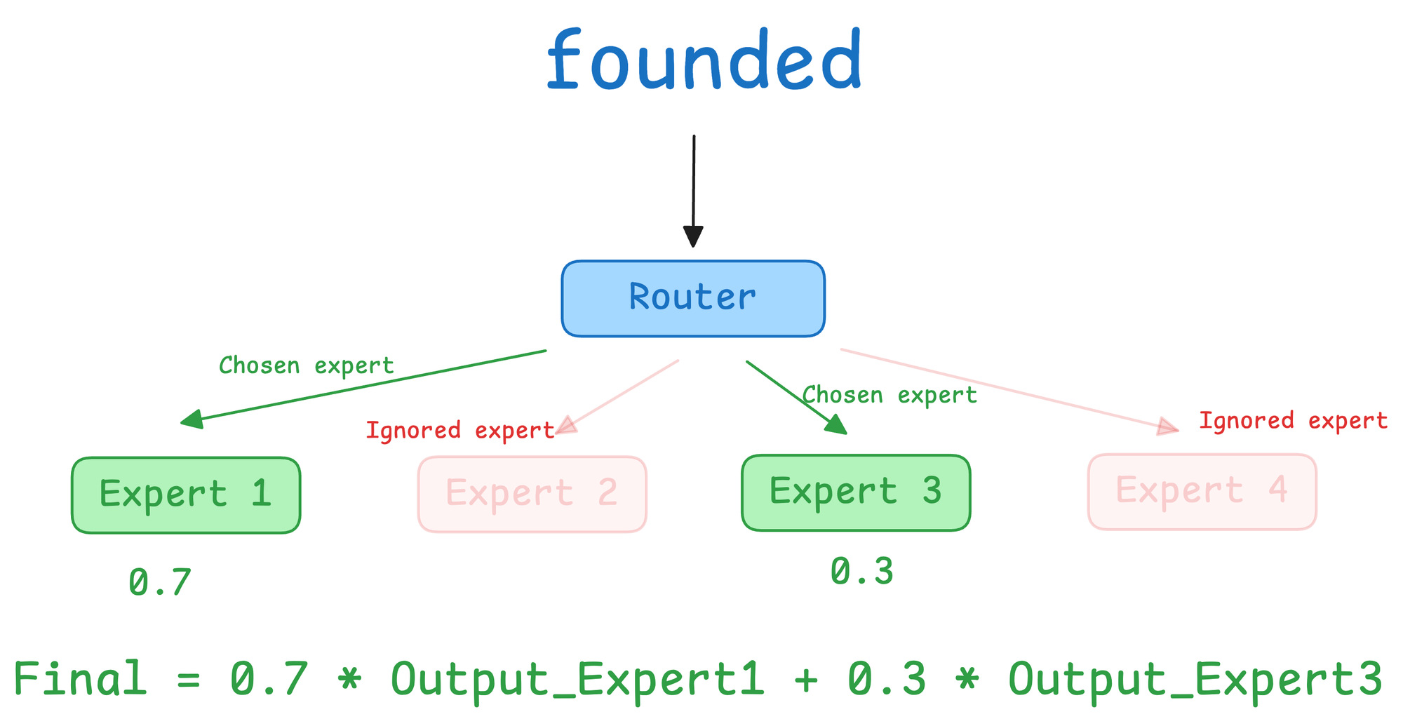
For example, imagine our model processing the sentence “Facebook was founded.”

When the MoE layer sees the token “was”, the router might determine that Expert 2 and Expert 4 are the best specialists for this token.

It gives, say, a 70% weight to Expert 1 and 30% to Expert 3.

Only those two experts get to work, while Experts 2 and 4 are ignored for “was”.

The model then combines the outputs of Experts 1 and 3 (weighted 0.7 and 0.3) to form the final output for that token.

In the next token “founded”, the router might choose a different set of experts, and so on. This dynamic routing is the key idea of MoE.

For instance, as shown in the figure above for the router mechanics on the token “was”, the router examines the input “was” and selects two experts (out of four) as the top performers for this token. In this illustration, Expert 1 and Expert 3 are chosen with weights 0.7 and 0.3, respectively.

Experts 1 and 3 are ignored (dashed outlines) for this token. Only Expert 1 and 3 compute their outputs, which will later be combined by the router’s weights. By activating just a couple of experts per token, the model saves computation.

Analogy #2 to understand MoEs

If you followed our AI Agents crash course, you already know the power of breaking a monolithic agent into specialized components, specifically a research agent, writer agent, and so forth, each with their own role in a coordinated system.

MoE takes a similar leap.

Think of a standard Transformer as a single-agent system. It’s like hiring one really smart generalist to do everything, write code, analyze data, design UI, write documentation.

MoE is the multi-agent version of model design. Instead of one generalist, you build a team of specialists, one expert in math, one in writing, another in reasoning, and you add a router to decide who gets what input.

Not everyone gets activated every time. Just like in multi-agent systems, only the most relevant experts are called in based on the task.

This produces a more compute-efficient, specialization-driven intelligence with sparse activation, ensuring you get the benefits of scale without paying the full cost each time.

Token prediction steps

To understand how token prediction works inside a Mixture-of-Experts (MoE) Transformer, let’s walk through what happens under the hood when the model is given the prompt:

“Facebook was founded”

We’ll assume word-level tokenization and a vocabulary that maps:

Let’s say we feed this sequence to the model with the goal of predicting the next word (e.g., “in”, “by”, “in 2004”, etc.).

Here’s how the model processes it, step by step:

Step 1) Embedding Layer

Each token is converted to an embedding, which is a dense vector that captures semantic meaning. So the model maps:

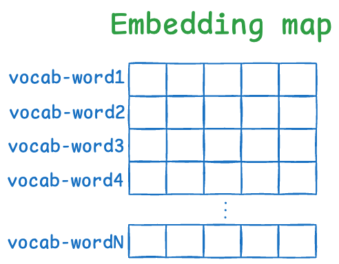
• “Facebook” → vector F (e.g., a 128-dimensional vector)
• “was” → vector W
• “founded” → vector D

These embeddings are also enriched with positional information via RoPE (rotary positional encoding), so the model knows “Facebook” comes first, “was” second, and so on.

Step 2) Masked Self-Attention

The embeddings go through a self-attention mechanism, where each word can look at others in the sequence to gather context.

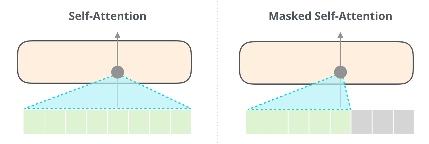
For example:

• “founded” attends to “was” and “Facebook”
• “was” attends to “Facebook”

After this, each token’s vector now encodes context. The vector for “founded” might now reflect a contextualized meaning like:

“This word follows a proper noun (‘Facebook’) and a past-tense verb (‘was’), so probably it's a past participle.”

Step 3) MoE Feed-Forward Layer

This is where things get interesting.

Instead of sending “founded” through a single feed-forward layer, the model passes it to a router, which is a lightweight neural network that decides which experts (sub-networks) should process it.

Let’s say we have 4 experts:

• Expert 1: good at verbs
• Expert 2: good at dates and numbers
• Expert 3: good at proper nouns and entities
• Expert 4: good at temporal phrases

The router takes the context-aware vector of “founded” and assigns weights to each expert. For example:

• Expert 1: 0.7
• Expert 3: 0.3
• (Experts 2 and 4 are ignored)

Only these two experts are activated. Each processes the “founded” vector through its own MLP and produces an output. The final output is a weighted combination:

This output becomes the representation for the word “founded” after the MoE layer.

Step 4) Final Projection → Vocabulary Logits

Once all tokens pass through the stack of Transformer blocks (each with self-attention and MoE), the final vector for the last token (“founded”) is used to predict the next token.

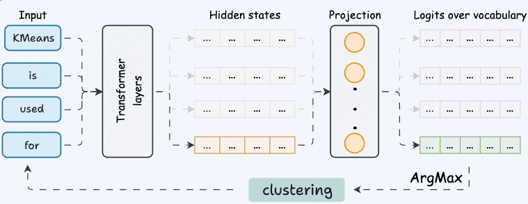
This is done via a final linear layer (a projection from embedding dimension to vocabulary size). The output is a logits vector, a score for every possible word in the vocabulary.

We apply softmax to turn these logits into probabilities. Let’s say the model predicts:

"in"       → 38%  
"by"       → 21%  
"2004"     → 14%  
"Mark"     → 9%  
"the"      → 6%  
... (rest of vocab)

The most probable next word is “in”.

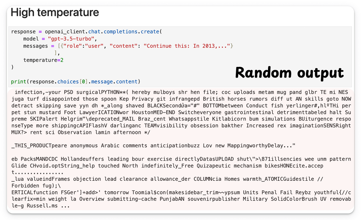
Step 5) Sample or Argmax

At inference time, we can either:

• Sample: pick the next word based on the probability distribution (adds variety),
• Argmax: pick the word with the highest probability (more deterministic).

The chosen word is appended to the prompt, and the whole process repeats to predict the next word after that.

Sampling is controlled with Temperature, which we covered here:

What is Temperature in LLMs?

Predictable ↔ Random.

Daily Dose of Data ScienceAvi Chawla

So to recap, for each token:

1. It's embedded into a vector with positional info.
2. It attends to previous tokens to gain context.
3. It is passed to a router that picks the top experts.
4. Only those experts are activated, making computation sparse.
5. The outputs from the experts are combined into a final vector.
6. The last token’s final vector is used to predict the next token.

Now that we understand what goes into a single token prediction, it's time for us to get into the implementation.

By the end of this tutorial, you will understand how to implement a simplified MoE Transformer language model from scratch using PyTorch.

We’ll build all the pieces step by step, including tokenization, embedding layers, self-attention with positional encodings, the MoE layer with multiple experts, normalization, and residual connections, and finally the training loop and text generation.

The style will be hands-on and conversational. We’ll print shapes and intermediate steps in the code to illuminate what’s happening under the hood, so you can follow along easily. Let’s get started!

Implementation

Now that we’ve covered the architecture and all its key building blocks, which include embeddings, RoPE, self-attention, and the Mixture-of-Experts (MoE) layer, it's time to bring everything together.

In this section, we'll build a complete end-to-end language model inspired by the core principles of LLaMA 4.

The focus will be on showing how the MoE component integrates into the Transformer pipeline, not just theoretically, but through a fully working mini-implementation.

We’ll follow a bottom-up approach where every stage of the pipeline is exposed:

• Each token gets embedded,
• Positional context is injected through rotary encodings,
• Self-attention allows tokens to learn from one another,
• MoE layers route each token to the right subset of experts,
• And finally, the model learns to predict the next word.

You can download the code below: