11 Powerful Techniques To Supercharge Your ML Models
Take your ML models to the next level with 11 lesser-known techniques.
Many machine learning engineers and data scientists very quickly pivot to building a different type of model when they don't get satisfying results with one kind of model.
At times, we do not fully exploit all the possibilities of existing models and continue to move towards complex models when minor tweaks in simple models can achieve promising results.
Over the course of building so many ML models, I have utilized various techniques that uncover nuances and optimizations we could apply to significantly enhance model performance without necessarily increasing the model complexity.
Thus, in this article, I will share 11 such powerful techniques that will genuinely help you supercharge your ML models so that you extract maximum value from them.
I provide clear motivation behind their usage, as well as the corresponding code, so that you can start using them right away.
Let’s begin!
#1) Robustify Linear Regression
The issue with regression models
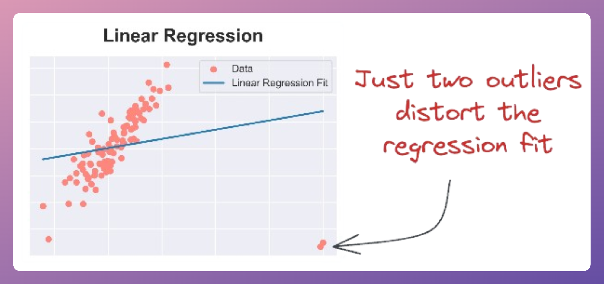
The biggest problem with most regression models is that they are sensitive to outliers.
Consider linear regression, for instance.
Even a few outliers can significantly impact Linear Regression performance, as shown below:
And it isn’t hard to identify the cause of this problem.
Essentially, the loss function (MSE) scales quickly with the residual term (true-predicted).
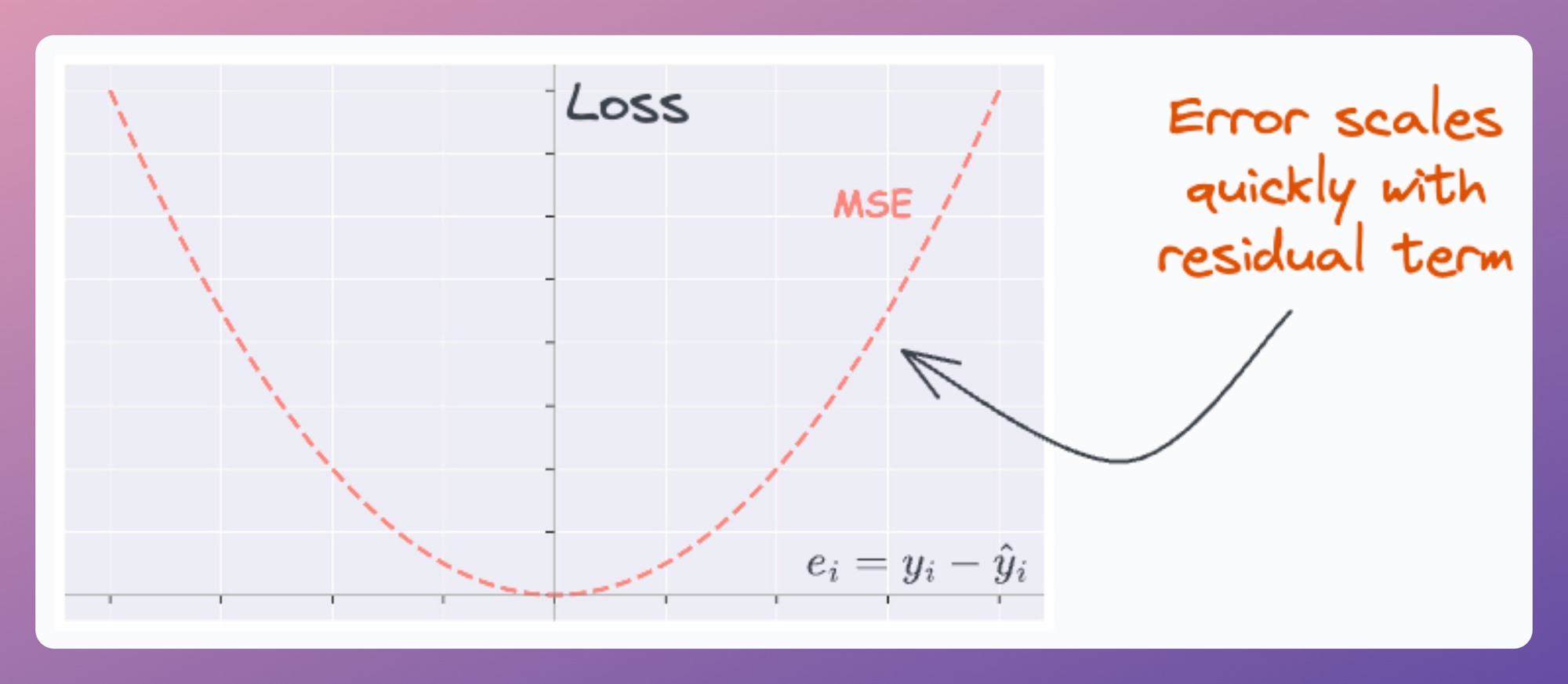
Thus, even a few data points with a large residual can impact parameter estimation.
Huber regression
Huber loss (used by Huber Regression) precisely addresses this problem.
In a gist, it attempts to reduce the error contribution of data points with large residuals.
How?
One simple, intuitive, and obvious way to do this is by applying a threshold (δ) on the residual term:
- If the residual is smaller than the threshold, use MSE (no change here).
- Otherwise, use a loss function that has a smaller output than MSE — linear, for instance.
This is depicted below:
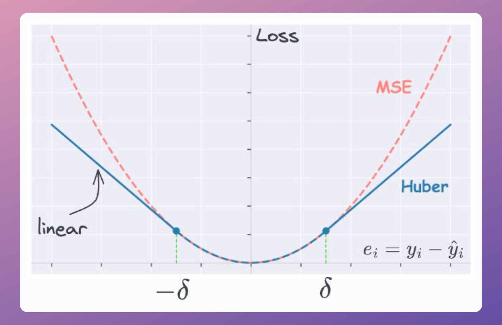
- For residuals smaller than the threshold (δ) → we use MSE.
- Otherwise, we use a linear loss function, which has a smaller output than MSE.
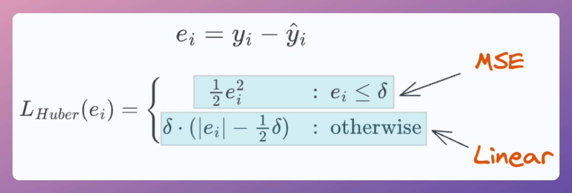
Mathematically, Huber loss is defined as follows:
Experiment
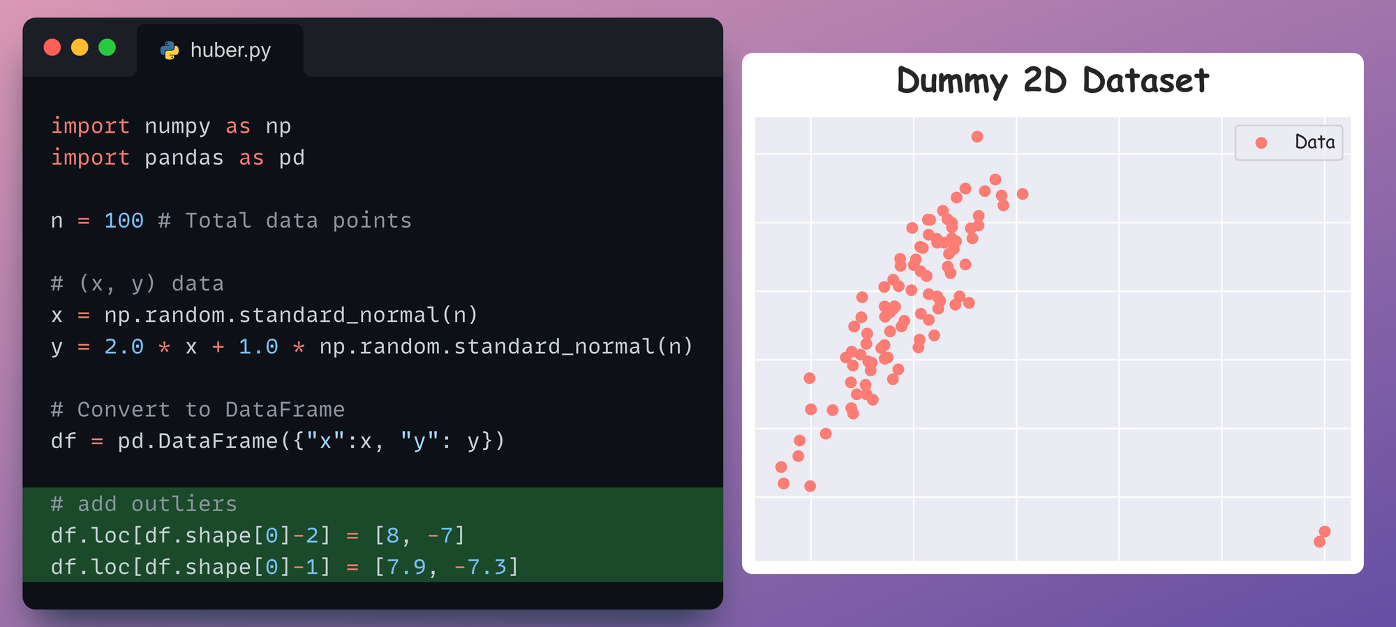
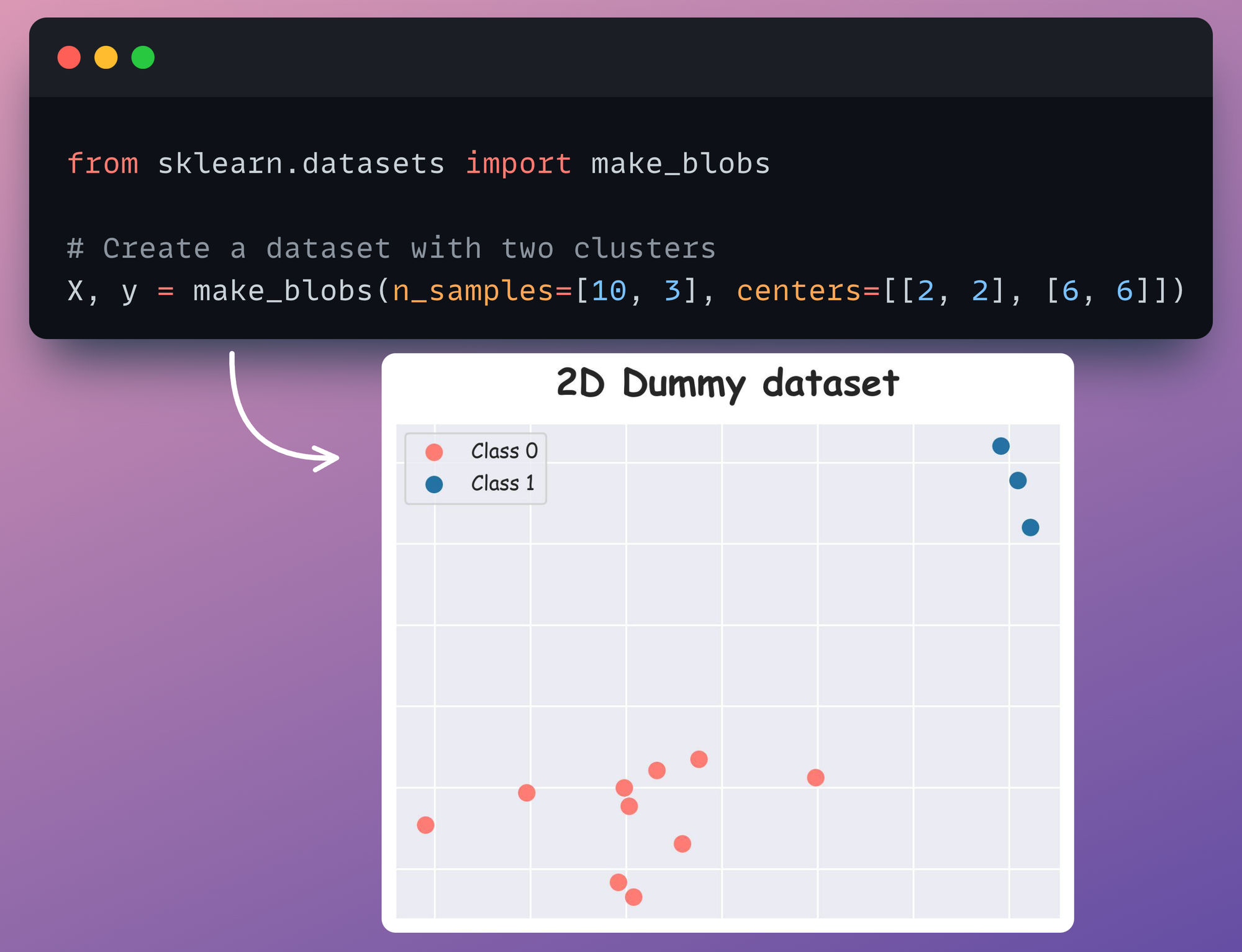
For instance, consider the 2D dummy dataset again which we saw earlier:
Currently, this dataset has no outliers, so let’s add a couple of them:
As a result, we get the following dataset:
Let’s fit a linear regression model on this dataset:
Next, we visualize the regression fit by plotting the y_pred values as follows:
This produces the following plot:
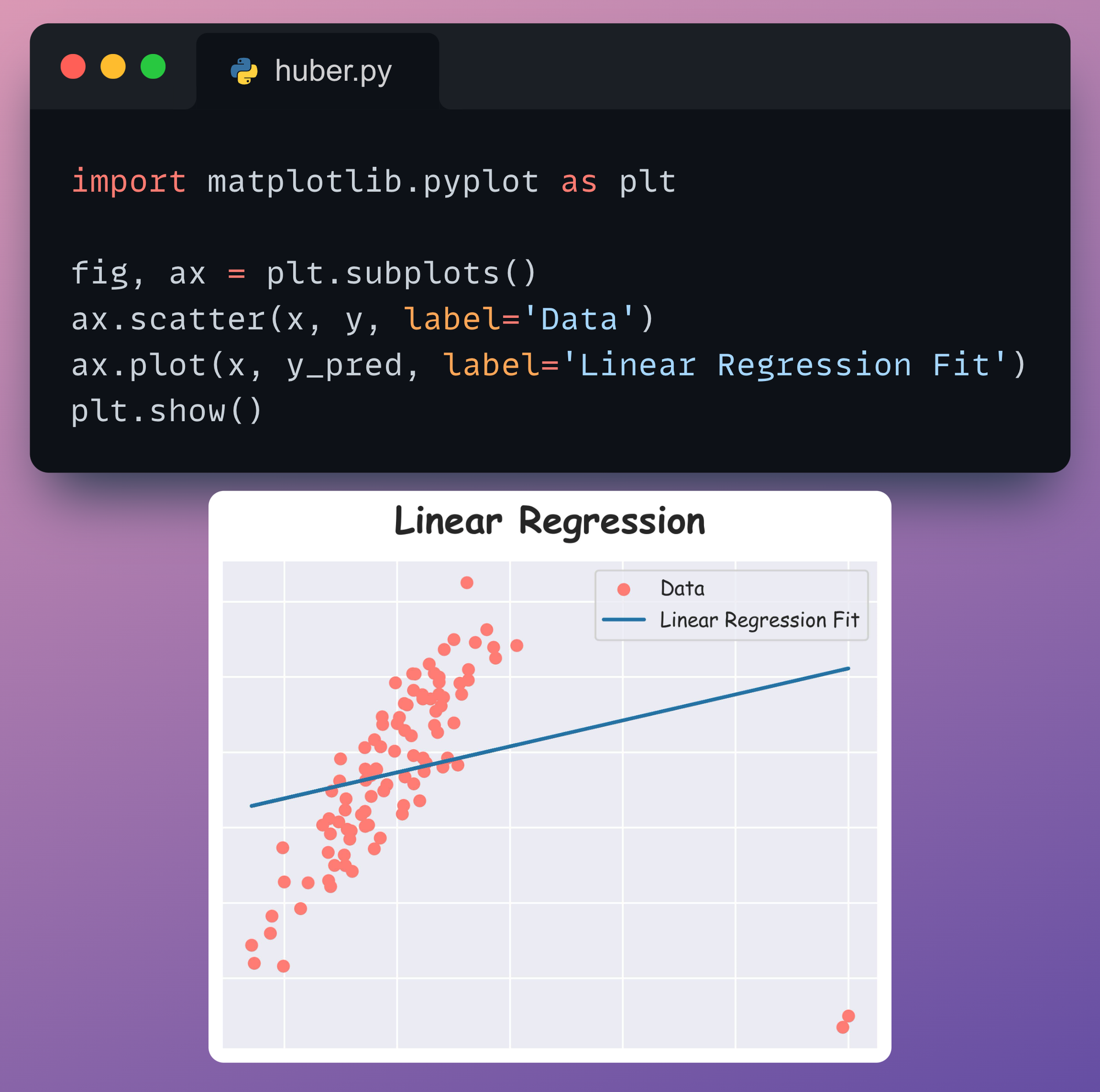
It is clear that the Linear Regression plot is affected by outliers.
Now, let’s look at the Huber regressor, which, as discussed earlier, uses a linear penalty for all residuals greater than the specified threshold $\delta$.
To train a Huber regressor model, we shall repeat the same steps as before, but this time, we shall use the HuberRegressor class from sklearn.
As a result, we get the following regression fit.
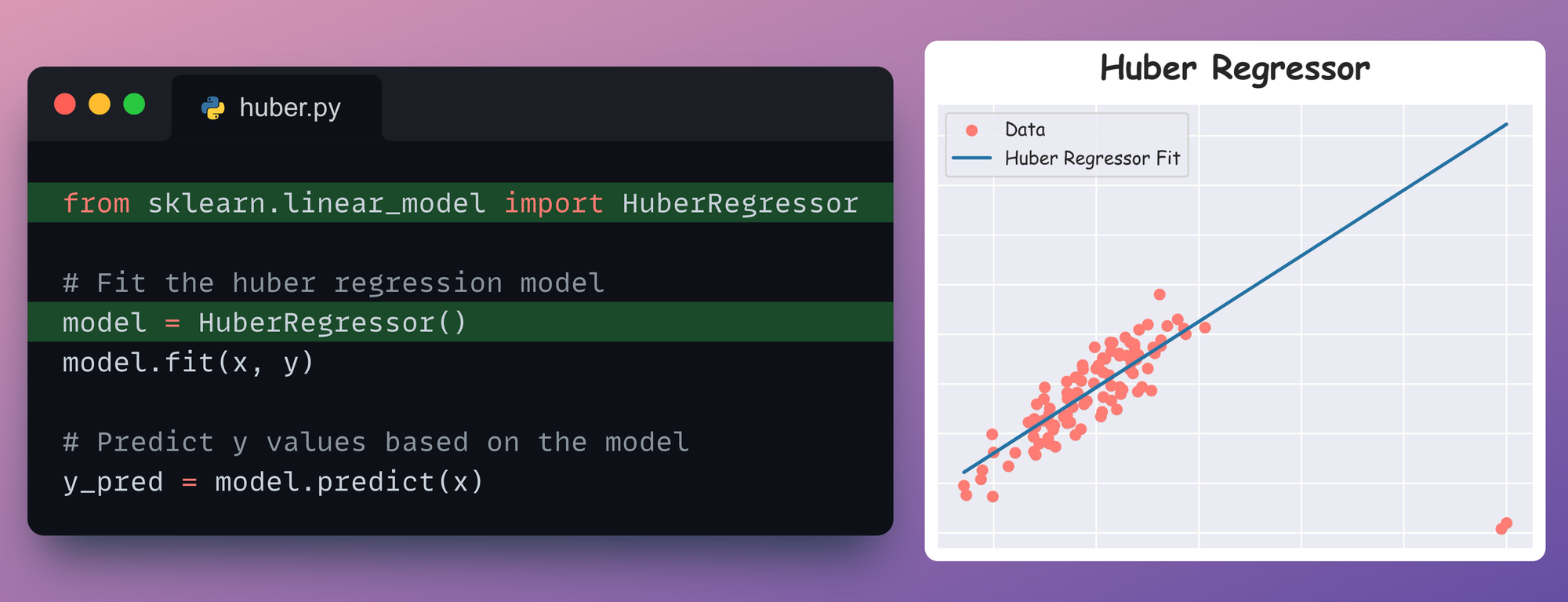
It’s clear that Huber regression is more robust.
How to determine δ?
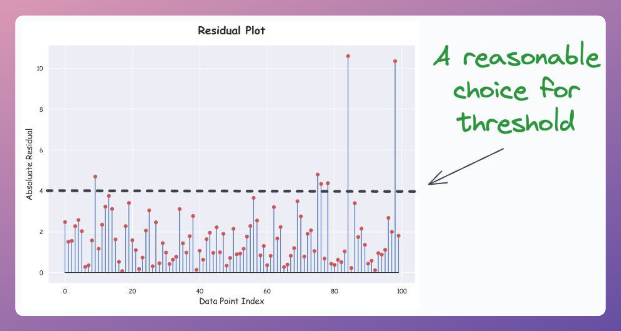
While trial and error is one way, creating a residual plot can be quite helpful. This is depicted below:
Here’s how we create it:
- Step 1) Train a linear regression model as you usually would on the outlier-included dataset.
- Step 2) Compute the absolute value of residuals (=true-predicted) on the training data.
- Step 3) Plot the absolute
residualsarray for every data point.
As a result, we get the following plot:
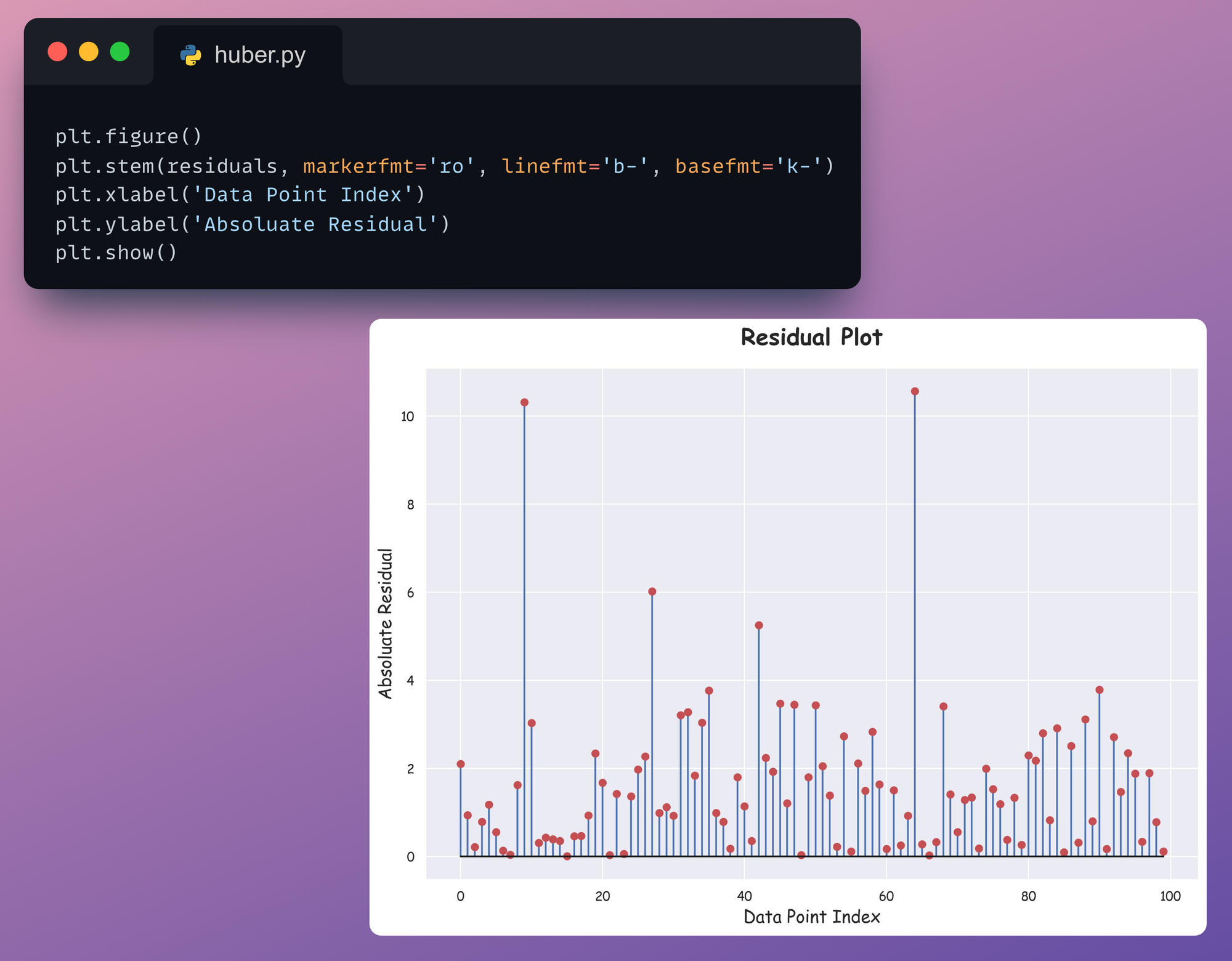
Based on the above plot, it appears that $\delta=4$ will be a good threshold value.
One good thing is that we can create this plot for any dimensional dataset. The objective is just to plot (true-predicted) values, which will always be 1D.
Overall, the idea is to reduce the contribution of outliers in the regression fit.
#2-3) Supercharge kNN Models
Issue with kNNs
One of the things that always makes me a bit cautious and skeptical when using kNN is its HIGH sensitivity to the parameter k.
To understand better, consider this dummy 2D dataset below. The red data point is a test instance we intend to generate a prediction for using kNN.
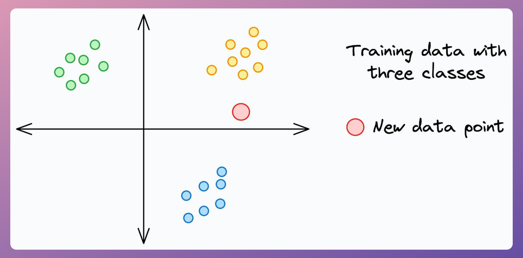
Say we set the value of k=7.
The prediction for the red instance is generated in two steps:
- First, we count the
7nearest neighbors of the red data point. - Next, we assign it to the class with the highest count among those 7 nearest neighbors.
This is depicted below:
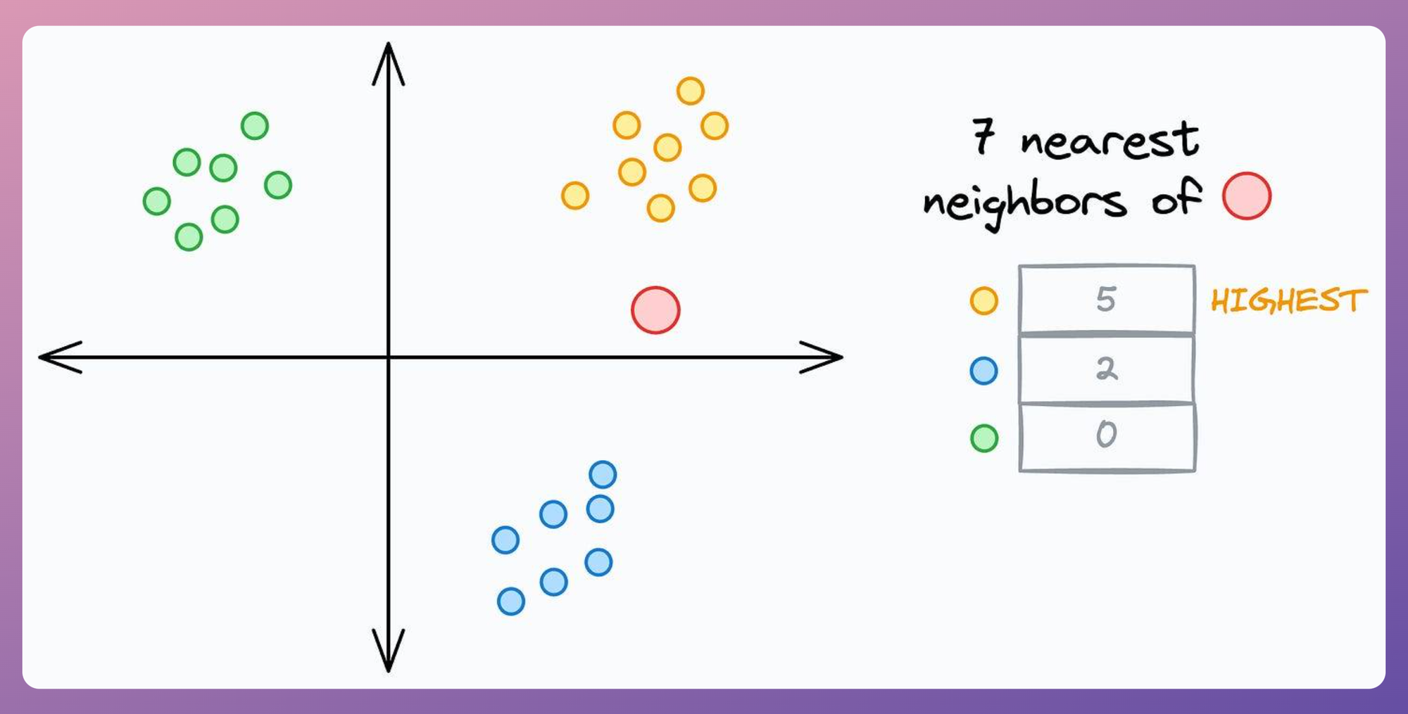
The problem is that step 2 is entirely based on the notion of class contribution — the class that maximally contributes to the k nearest neighbors is assigned to the data point.
But this notion fails miserably at times, especially when we have a class with few samples.
For instance, as shown below, with k=7, the red data point can NEVER be assigned to the yellow class, no matter how close it is to that cluster:
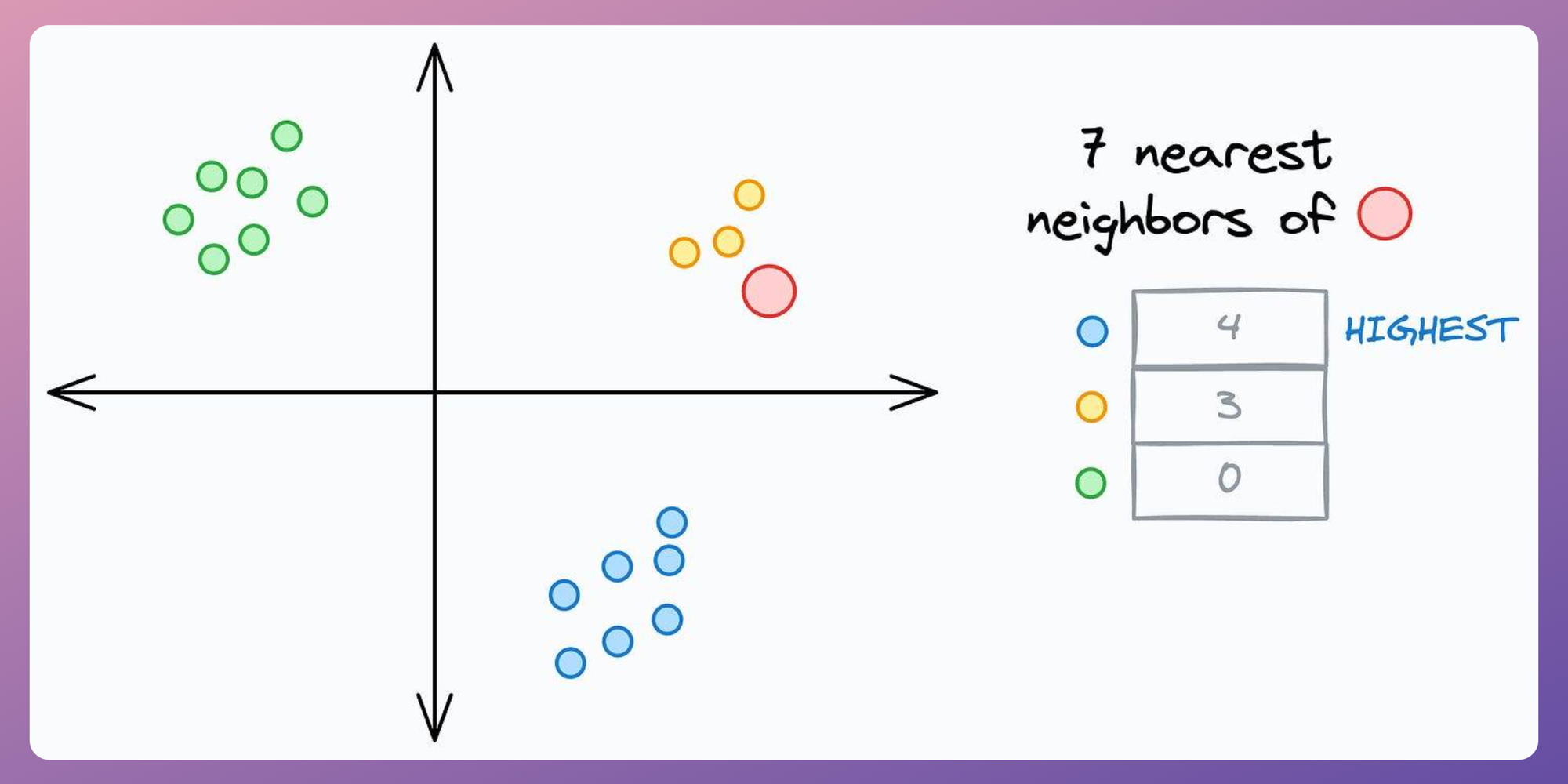
While it is easy to tweak the hyperparameter k visually in the above demo, this approach is infeasible in high-dimensional datasets.
There are two ways to address this.
Solution #1: Used distance-weighed kNN
Distance-weighted kNNs are a much more robust alternative to traditional kNNs.
As the name suggests, in step 2, they consider the distance to the nearest neighbor.
As a result, the closer a specific neighbor is, the more impact it will have on the final prediction.
For instance, consider this 2D dummy dataset:
Now, consider a dummy test instance:
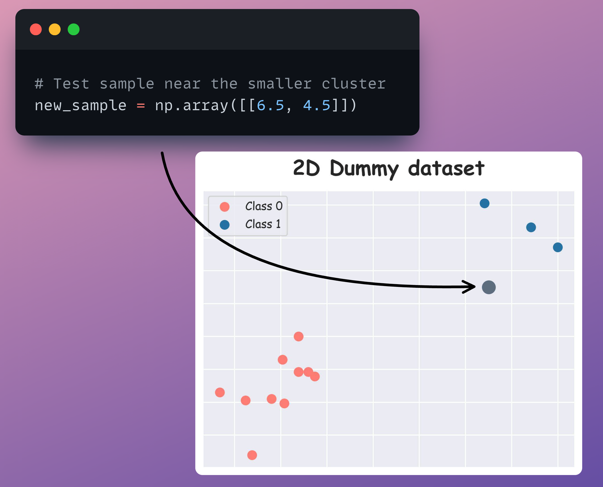
Training a kNN classifier under the uniform (count-based) strategy, the model predicts the class 0 (the red class in the above dataset) as the output for the new instance:
However, the distance-weighted kNN is found to be more robust in its prediction, as demonstrated below:
This time, we get Class 1 (the blue class) as the output, which is correct.
As per my observation, a distance-weighted kNN typically works much better than a traditional kNN. And this makes intuitive sense as well.
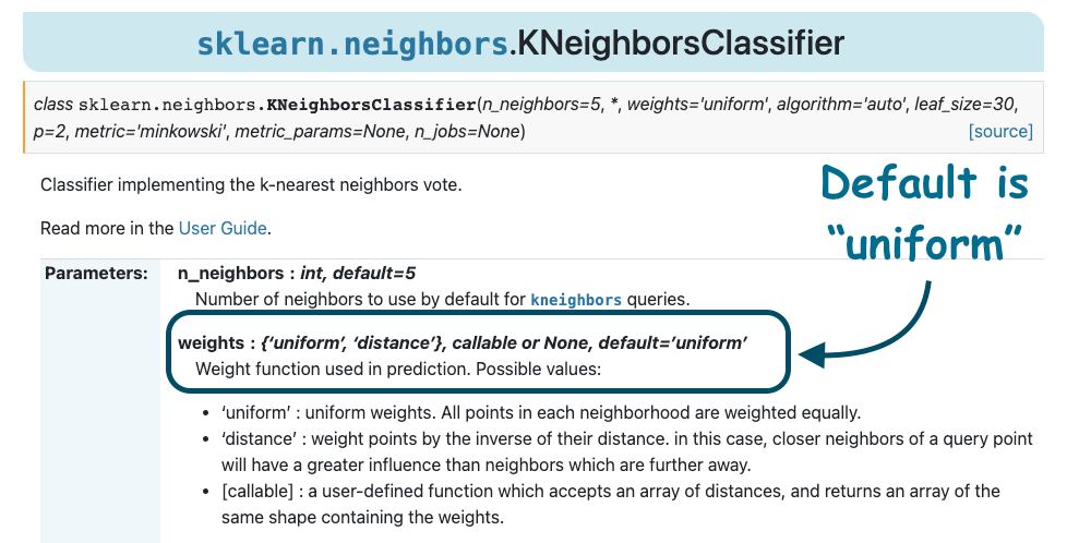
Yet, this may go unnoticed because, by default, the kNN implementation of sklearn considers uniform weighting.
Solution #2: Dynamically update the hyperparameter k
Recall the diagram I started this kNN discussion with:
Here, one may argue that we must refrain from setting the hyperparameter k to any value greater than the minimum number of samples that belong to a class in the dataset.
Of course, I agree with this to an extent.
But let me tell you the downside of doing that.
Setting a very low value of k can be highly problematic in the case of extremely imbalanced datasets.
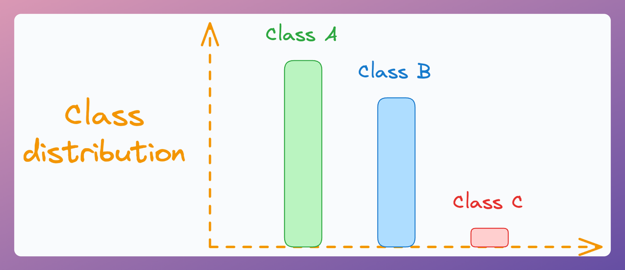
To give you more perspective, I have personally used kNN on datasets that had merely one or two instances for a particular class in the training set.
And I discovered that setting a low of k (say, 1 or 2) led to suboptimal performance because the model was not as holistically evaluating the nearest neighbor patterns as it was when a large value of k was used.
In other words, setting a relatively larger value of k typically gives more informed predictions than using lower values.
But we just discussed above that if we set a large value of k, the majority class can dominate the classification result:
To address this, I found dynamically updating the hyperparameter k to be much more effective.
More specifically, there are three steps in this approach.
For every test data point:
- Step 1) Begin with a standard value of
kas we usually would and find theknearest neighbors. - Step 2) Next, update the value of the
kas follows:- For all unique classes that appear in the
knearest neighbor, find the total number of training instances they have.
- For all unique classes that appear in the
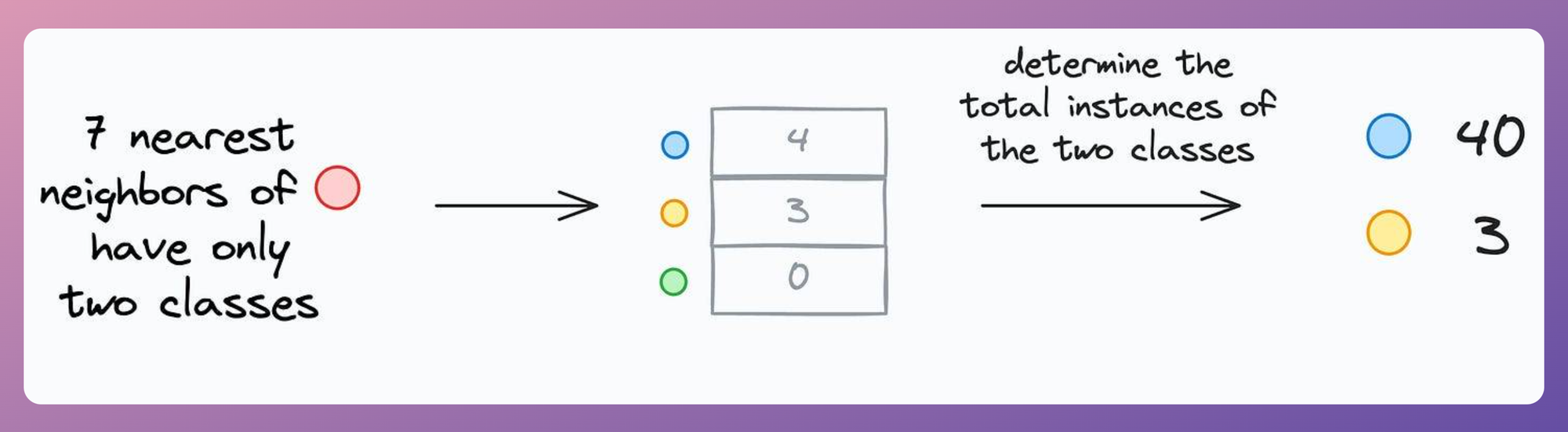
- Update the value of k to:
$$ \Large k' = min(k, 40, 3) $$
- Step 3) Now perform majority voting only on the first
k'neighbors only.
This makes an intuitive sense as well:
- If a minority class appears in the top
knearest neighbor, we must reduce the value ofkso that the majority class does not dominate. - If a minority class DOES NOT appear in the top
knearest neighbor, we will likely not update the value ofkand proceed with a holistic classification.
I used this approach in a couple of my research projects. If you want to learn more, here’s my research paper: Interpretable Word Sense Disambiguation with Contextualized Embeddings.