Model Deployment: Serialization, Containerization and API for Inference
MLOps Part 11: A practical guide to taking models beyond notebooks, exploring serialization formats, containerization, and serving predictions using REST and gRPC.
Recap
Before we dive into Part 11 of this MLOps and LLMOps crash course, let’s quickly recap what we covered in the previous part.
Part 10 concluded the discussion on the modeling phase of the machine learning system lifecycle.
There, we explored model compression techniques and ONNX for efficient and optimized modeling.
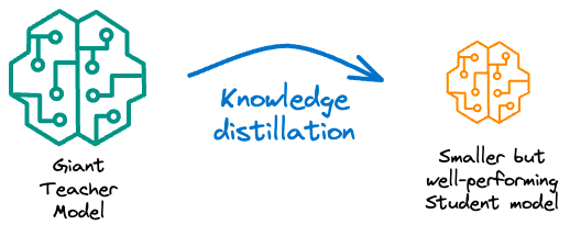
We began by understanding the knowledge distillation (KD) through concept and a practical hands-on example.
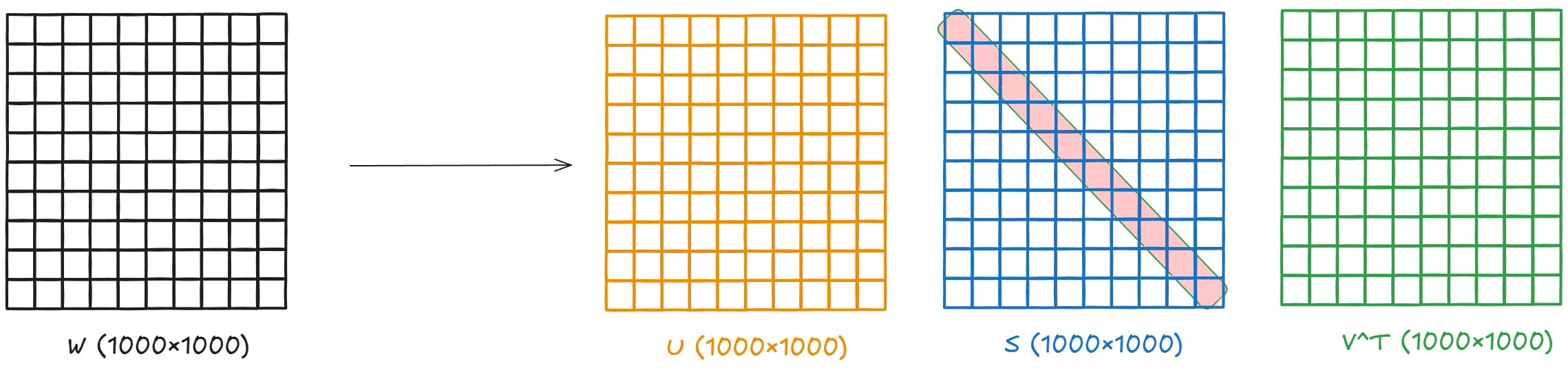
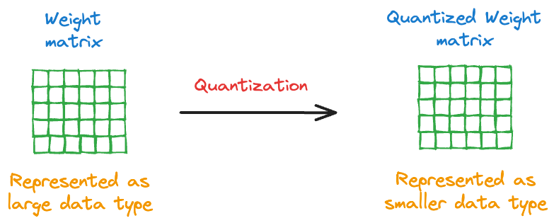
Similar to KD, we explored low-rank factorization and quantization through concepts and hands-on exercises.
Finally, we explored ONNX and ONNX runtime, understanding its architecture and framework-agnostic intermediate representation.

If you haven’t explored Part 10 yet, we strongly recommend going through it first, since it sets the foundations and flow for what's about to come.
Read it here:
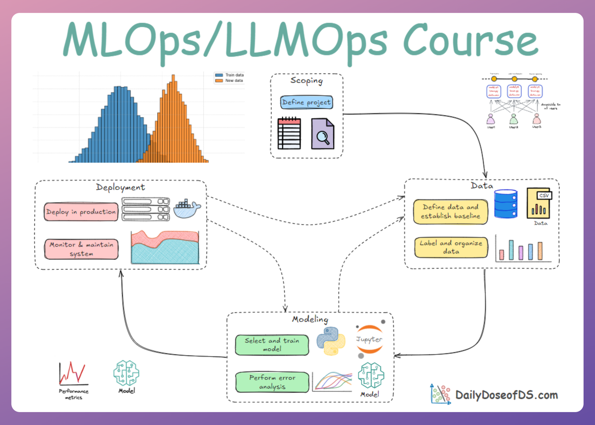
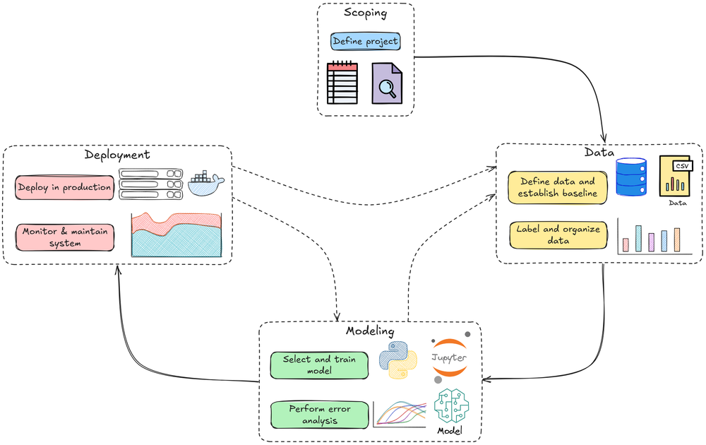
In this chapter, we'll move ahead and dive deep into the deployment phase of the MLOps lifecycle, discussing it from a systems perspective.

Modern machine learning systems don’t deliver value until their models are reliably deployed and monitored in production. Hence, in this and the next few chapters, we’ll discuss how to package, deploy, serve, and monitor the models in a robust manner.
In this chapter, we'll cover:
- Model packaging formats
- Containerization
- Serving APIs
As always, every idea and notion will be backed by concrete examples, walkthroughs, and practical tips to help you master both the idea and the implementation.
Let’s begin!
Introduction
The journey of a machine learning model from a Jupyter Notebook to a production system is one of the most challenging aspects of the MLOps lifecycle.
It represents a fundamental shift in thinking, from the isolated, experimental world of a data scientist to the complex, interconnected, and unforgiving reality of a systems engineer.
This initial chapter on model deployment aims to reframe the problem of deployment, moving beyond the simple act of running a model to embrace the discipline of building a reliable, scalable, and maintainable software system.
Model deployment fundamentals
Model deployment means taking a model out of the research/training environment (e.g., your notebook or development server) and making it run as a service accessible to other systems.
In practical terms, this involves serializing the model into a portable format, packaging it (often in a container), and exposing it via an API.
This section covers the basics:
- choosing a model format
- containerizing with Docker
- building a web API
- understanding different ways clients might interact with the model
Packaging and serialization formats
Packaging a model refers to saving or exporting the trained model in a format that can be loaded and executed in another environment. This is often called model serialization.
The format you choose affects portability, compatibility, and ease of deployment.
Let’s examine a few common formats:
Pickle
Pickle (.pkl) is the classic Python serialization format. Using Python’s built-in pickle module, you can dump a model object to disk and load it later.
This works well for many scikit-learn models or simple Python objects.
To consider the plus points: it’s easy (one line to pickle.dump(model) and pickle.load()), and it preserves Python objects directly.
But there are a few downsides as well: pickle is Python-specific (you can’t easily load a pickle in non-Python environments) and can be insecure if you load untrusted pickled data (pickle can execute arbitrary code on load).
Joblib

Joblib (.joblib) is effectively a variant of pickle optimized for NumPy arrays. Scikit-learn often recommends it for model persistence because it handles large numpy arrays efficiently.
Usage is similar (joblib.dump(model) and joblib.load()), and it’s generally faster and more memory-efficient for big models than raw pickle. Like pickle, it’s Python-only.
HDF5
HDF5/Keras (.h5) is for deep learning models (TensorFlow/Keras), the Hierarchical Data Format (.h5) or TensorFlow’s SavedModel format is common.
model.save('model.h5') in Keras stores the architecture and weights together. This format is cross-platform (doesn’t require Python specifically) and is supported by TensorFlow Serving. However, it’s mostly tied to the TensorFlow ecosystem.
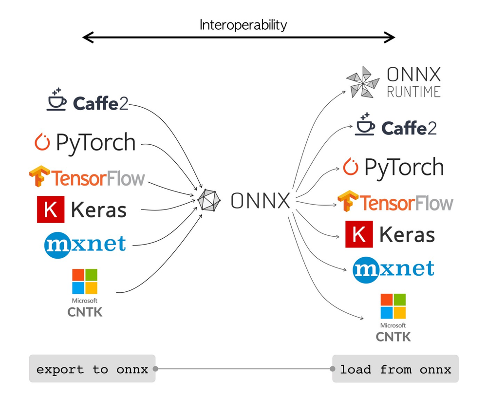
ONNX

ONNX (.onnx), as discussed earlier in the series, is an open standard for ML models. ONNX is framework-agnostic and designed for interoperability. You can convert models from PyTorch, TensorFlow, scikit-learn, etc., into ONNX format.
The advantage is that ONNX models can be loaded and executed in many environments via the ONNX Runtime, including C++ programs, mobile devices, or other languages, without needing the original training code.
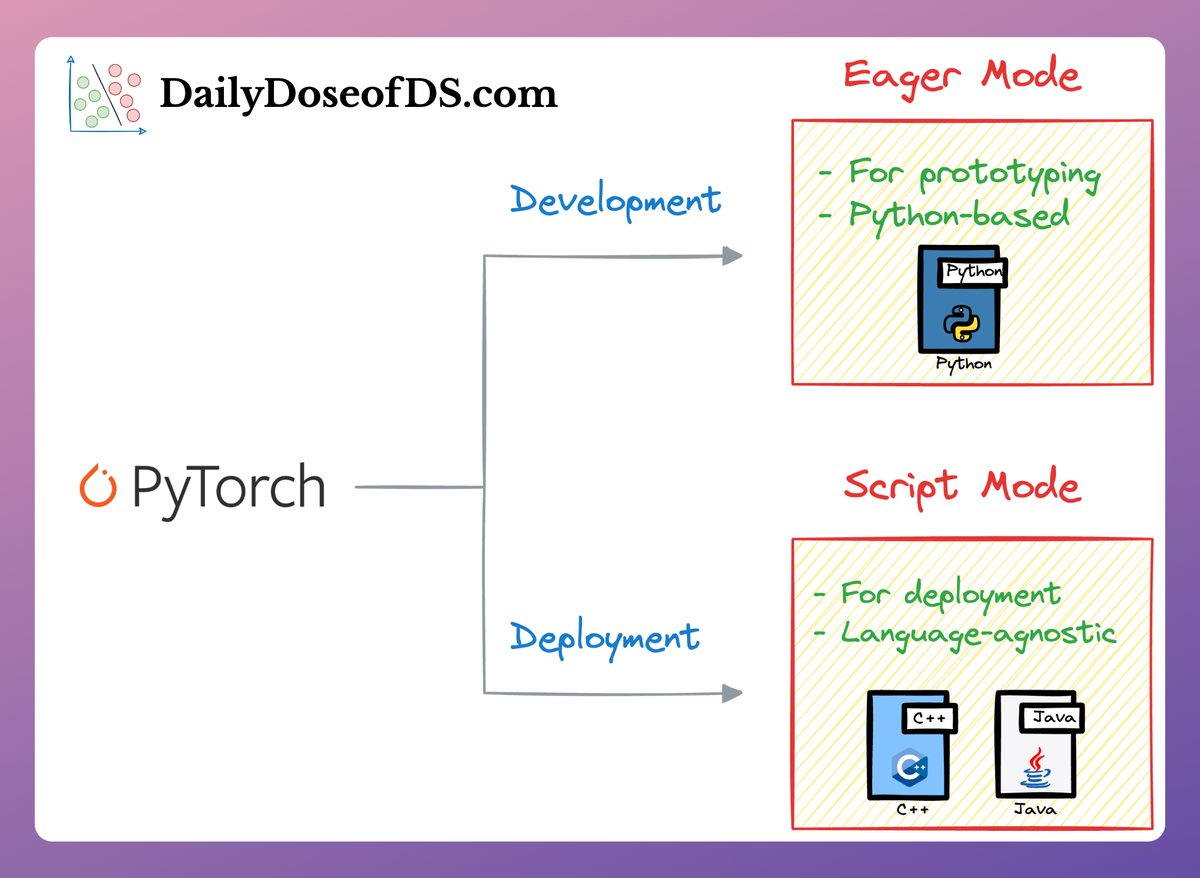
TorchScript
TorchScript (.pt or .pth) is PyTorch’s native model format. In PyTorch, you often save model weights as a .pt or .pth file (using torch.save on the state_dict). Loading it requires the model’s code structure to rebuild the neural net and load weights.
Alternatively, PyTorch’s TorchScript allows saving the model as a scripted or traced module, which can then run independently of Python (for example, in a C++ runtime or on mobile).
TorchScript is great for deploying PyTorch models in production because you can avoid Python and achieve optimized execution. However, it’s PyTorch-specific and may require writing some PyTorch code to script/trace the model.
If you want to learn more, this part covers it:
Now that we know the major formats, it is important to understand that, in practice, there is no one-size-fits-all format.
The choice depends on your framework and deployment requirements. For quick Python-only deployments (e.g., internal tools), pickle/joblib might suffice.
For long-term production services, export to a neutral format like ONNX or a framework-specific production format (SavedModel, TorchScript) that is optimized for serving. Indeed, exporting is often required when handing off a model to a different team or environment for deployment.
For example, a data scientist trains a model in Python, but an engineering team will deploy it in a Java service; using ONNX or another interoperable format is critical.
Now that we’ve covered model serialization, let’s move on to the next step in the machine learning workflow.
Containerization with Docker
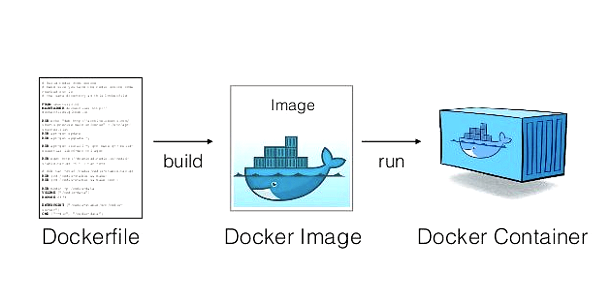
Once the model is serialized, how do we actually deploy it on a server? In modern MLOps, the answer is almost always containers.
Containerization (e.g., using Docker) allows you to package the model and its code, along with all required libraries and dependencies, into a self-contained unit that can run anywhere (on your laptop, on a cloud VM, in a Kubernetes cluster, etc.).

This solves the classic “it works on my machine” problem by ensuring the environment is consistent. By containerizing the model server, you encapsulate the Python version, libraries (pandas, numpy, scikit-learn, etc.), and even the model file itself inside an image.
In practice, you’ll write a Dockerfile that starts from a base image (e.g., a Python base image), copies your model and code, installs dependencies, and sets the command to launch your model service.
Containers make scaling and deployment easier because they provide a standard interface: as long as a server can run Docker (or you have Kubernetes, etc.), it can run your model container. In fact, container orchestration (discussed later) relies on this uniform deployable unit.
This approach is also cloud-agnostic: you can run the same container on AWS, GCP, Azure, or on-premise. It encapsulates the model runtime environment, ensuring consistency between dev, staging, and prod.
As an industry best practice, most production ML services are containerized, whether you manage it yourself or use a cloud service under the hood.
Serving models via FastAPI (building a prediction API)
With the model packaged and containerized, the next step is to expose it via an API so that other systems (or users) can request predictions. A common pattern is to wrap the model inference in a web service.
For this, we can use FastAPI (a modern, high-performance web framework for Python) to create prediction APIs. FastAPI is popular for ML deployment because it’s easy to use and very fast (built on ASGI/UVicorn). Also, by containerizing FastAPI-built services, we can deploy them anywhere.

Why FastAPI?
FastAPI has rapidly gained traction in the Python community for several key reasons that make it particularly well-suited for ML model serving:
- High performance: Built on top of Starlette (for the web parts) and Pydantic (for the data parts), FastAPI is one of the fastest Python frameworks available, comparable to NodeJS and Go. Its asynchronous support allows it to handle concurrent requests efficiently, which is crucial for a scalable prediction service.
- Automatic data validation: FastAPI uses standard Python type hints and the Pydantic library to define data schemas. It automatically validates incoming request data against these schemas, rejecting invalid requests with clear error messages. This eliminates a significant amount of boilerplate validation code and protects the ML model from receiving malformed input.
- Automatic interactive documentation: Out of the box, FastAPI generates interactive API documentation based on the OpenAPI (formerly Swagger) standard. This provides a user-friendly interface (accessible at
/docs) where developers can explore endpoints, see expected request and response formats, and even test the API directly from their browser. This dramatically simplifies API integration and debugging.
Overall, , makes it straightforward to go from a model.predict() function to a web API. In fact, deploying a simple model can be done in a few lines. The challenge is what comes next; ensuring this service can handle scale, reliability, and updates, which we will address in subsequent chapters.
API Communication: REST vs. gRPC
When building an API for model inference, two common communication protocols are:
- REST (usually over HTTP/1.1 with JSON)
- gRPC (a high-performance RPC framework using HTTP/2 and Protocol Buffers).
Each has pros and cons, and understanding them will inform your deployment choices:
REST
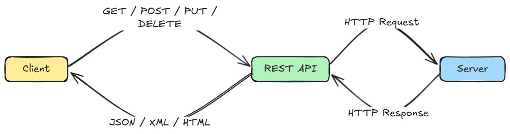
REST is an architectural style based on standard HTTP/1.1 methods (like GET, POST, PUT, DELETE) operating on resources identified by URLs.
It typically uses human-readable, text-based data formats like JSON. Its stateless nature means each request contains all the information needed to process it, making it highly scalable and loosely coupled.
Advantages:
- Very simple to implement and integrate
- JSON is human-readable
- Works natively with web infrastructure (browsers, gateways, etc.)
Drawbacks:
- JSON is text-based and verbose, which can be inefficient for large payloads
- HTTP/1.1 is half-duplex (one request, one response), so it can’t stream easily
Overall, for many ML use cases, where payloads might be small, like a few features, REST is perfectly fine and very convenient.
gRPC
gRPC is a more recent high-performance alternative, originally developed by Google. Instead of operating on resources, a gRPC client directly invokes methods on a server application as if it were a local object.

It leverages the modern HTTP/2 protocol, which allows for multiplexing, i.e., sending multiple requests and responses over a single, long-lived TCP connection, eliminating connection setup overhead and head-of-line blocking.
Data is serialized using Protocol Buffers (Protobufs), a highly efficient, language-neutral binary format.
With the benefit of a highly efficient, compact data exchange and full-duplex streaming support, gRPC can significantly outperform REST in terms of latency and throughput. Studies show gRPC can be several times faster than REST for the same data, due to binary encoding and lower overhead.
Advantages:
- Low latency, high throughput
- Built-in code generation (you define a
.protofile and gRPC generates client/server stubs)
- Streaming capabilities (a client or server can send a stream of messages rather than a one-shot request/response)
This makes gRPC well-suited for internal microservice communication or high-performance needs. For instance, a model serving thousands of predictions per second behind the scenes might use gRPC to communicate between services.
Drawbacks:
- Not human-readable (Protobuf binary can’t be easily inspected or manually crafted)
- Requires client support (though many languages have gRPC libraries)
- Not directly callable from a web browser (since browsers don’t natively speak gRPC without a proxy).
In practice, when to use which?
For external-facing services or quick integrations, REST is usually the default because of its simplicity and ubiquity. For example, in the case of, say, a fraud detection model, if the service is called directly by a front-end or mobile app, REST/JSON is an easy choice.
On the other hand, if the model is deployed as part of a larger microservice architecture where performance is critical, say, hundreds of microservices in a banking system calling each other; gRPC might be chosen for its efficiency.
For example, a fraud detection model might be one service called by a transaction processing service; using gRPC could reduce the latency added by the call and allow streaming multiple transaction checks in one connection if needed.
Comparison summary
| Feature | REST | gRPC |
|---|---|---|
| Protocol | HTTP/1.1, widely supported. HTTP/2 possible. | HTTP/2, enables multiplexing and efficiency. |
| Data Format | JSON (text-based, human-readable). | Protocol Buffers (compact binary). |
| Performance | Good, but higher latency due to JSON parsing. | High; lower latency and better throughput. |
| Streaming Support | Primarily unary request–response, but supports SSE, WebSockets. | Natively supports unary, server, client, and bidirectional streaming. |
| Coupling | Loosely coupled; independent client and server. | Tightly coupled; requires shared .proto file. |
| Ease of Debugging | Easy; JSON can be tested with curl, Postman, or browser. | Harder; binary requires grpcurl or special tools. |
| Common Use Cases |
- Public APIs - Web/mobile backends - Broad compatibility |
- Internal microservices - Real-time streaming - Low-latency systems |
Batch vs. real-time inference
Although we previously explored this topic in one of the initial chapters, since we are discussing deployment specifically here, it is important to revisit it, as it represents a critical architectural decision in the context of model deployment.
Both batch inference and real-time inference have distinct use cases and implications for how you deploy and monitor models. This choice is not merely a technical detail but a core product and business strategy decision.
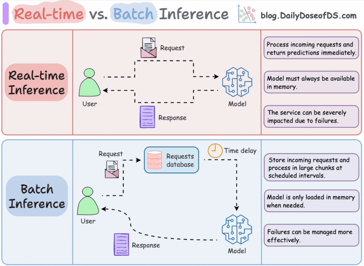
Real-time (online/synchronous) inference means the model is deployed as a live service, receiving individual requests (often via a REST or gRPC API) and returning predictions immediately (in milliseconds).
Real-time inference prioritizes low latency and high availability. The system must always be operational, and typically auto-scales to handle varying request volumes.
Batch inference (offline/asynchronous inference) involves running the model on a large collection of data all at once, usually on a schedule or triggered by some event. Here, latency per prediction is less critical; the goal is throughput and efficiency.
The key characteristics of batch inference are that it’s not user-facing in real time, can leverage heavy compute for a short period, and results are stored for later use rather than returned instantly to a user.
Because batch jobs can run without a live API, they often run on a separate infrastructure (e.g., a Cloud function triggered on a schedule, etc.) and can scale up resources (like using 100 CPU cores for 10 minutes) then shut down, which can be cost-efficient.
The decision of choosing one often comes down to the use case requirements. If a prediction is needed immediately in a user flow, you must do online serving. If predictions can be pre-computed, a batch might simplify the problem.
From a deployment perspective, batch jobs might be containerized as well but deployed to a job scheduler or pipeline (like Airflow/Prefect, Kubeflow Pipelines, cloud Data Pipeline services, etc.), whereas online models are deployed to a serving infrastructure (web servers, Kubernetes, etc.).
Now that we've covered the core concepts of this chapter, let's dive into a practical exercise on gRPC.
Hands-on: from training to gRPC API
Since we’ve already covered a FastAPI-based example in Chapter 2, we won’t repeat it here. Instead, we’ll focus on understanding gRPC through a hands-on demo.
If you missed the earlier FastAPI-based example, you can find the link below:

Objective
Imagine we have a Jupyter notebook/Python script where we trained a basic model, a linear regression one, that basically maps the simple relation $y = 2x$.
We want to expose a trained ML model as a gRPC API, allowing clients to call it remotely. This exercise simulates the journey of turning a data science prototype into a microservice.
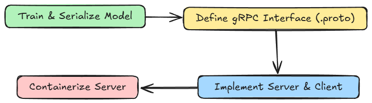
Steps to follow
- Train and serialize the model:
- Start by training the model in a notebook or Python script.
- Save the trained model to disk so it can be loaded later by the server.
- Define the gRPC interface (
.protofile)- Write a
.protofile that describes the service. - Specify the request and response message formats and the RPC method(s) (e.g.,
Predict). - This acts as a contract between the server and clients.
- Write a
- Implement the server and client
- Generate Python code from the
.protofile usinggrpcio-tools. - Implement the server that loads the serialized model and serves predictions via gRPC.
- Implement a simple client that connects to the server, sends requests, and displays responses.
- Generate Python code from the
- Containerize the server
- Write a
Dockerfileto package the server, model, and dependencies. - This ensures reproducibility and portability.
- In a real-world scenario, this container can be deployed on a platform (Kubernetes, cloud services, etc.).
- Write a
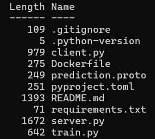
Project setup
The code and project setup we are using are attached below as a zip file. You can simply extract it and run uv sync command to get going. It is recommended to follow the instructions in the README file to get started.
Download this project's file below: