Data and Pipeline Engineering: Data Sources, Formats, and ETL Foundations
MLOps Part 5: A detailed walkthrough of data engineering for MLOps, covering data sources, format performance trade-offs, and ETL/ELT pipelines.
Recap
Before we dive into Part 5 of this MLOps and LLMOps crash course, let’s quickly recap what we covered in the previous part.
In Part 4, we extended our discussion on reproducibility and versioning into a hands-on exploration with Weights & Biases (W&B).

We began with an introduction to W&B, its core philosophy, and how it compares side-by-side with MLflow.
The key takeaway was clear: MLflow vs W&B isn’t about which is better, it’s about choosing the right tool for your use case.

From there, we went hands-on. We explored experiment tracking and versioning with W&B through two demos:
- Predictive modeling with scikit-learn, where we:
- logged metrics
- tracked experiments
- managed artifacts
- registered models
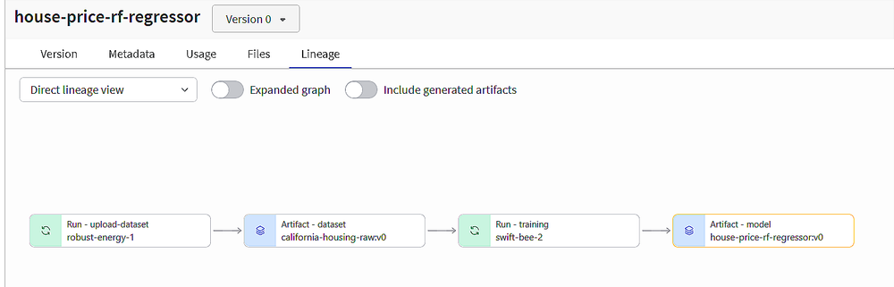
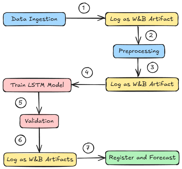
- Time series sales forecasting with PyTorch, where we learned about:
- building multi-step pipelines
- W&B’s deep learning integration
- logging artifacts
- checkpointing models
If you haven’t checked out Part 4 yet, we strongly recommend going through it first, since it sets the foundations and flow for what's about to come.
Read it here:
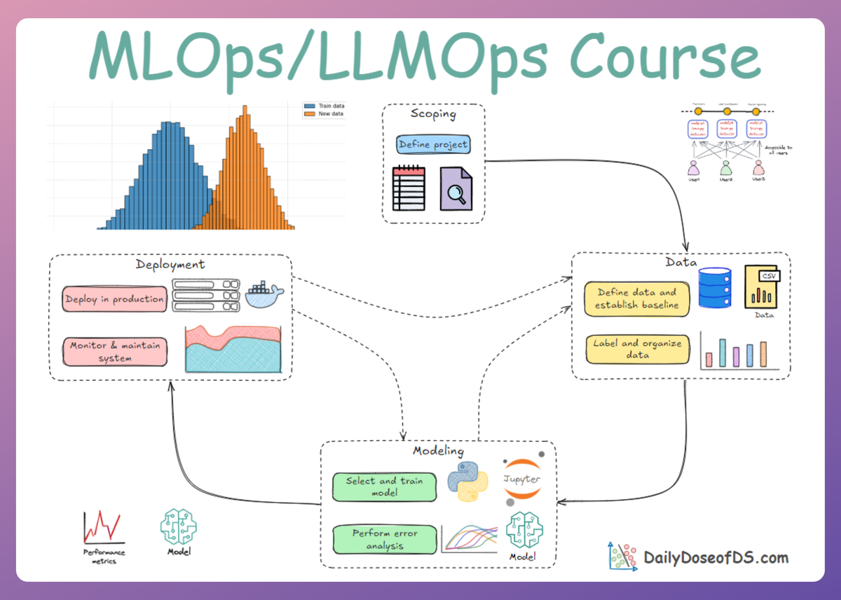
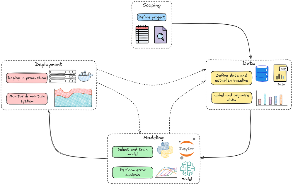
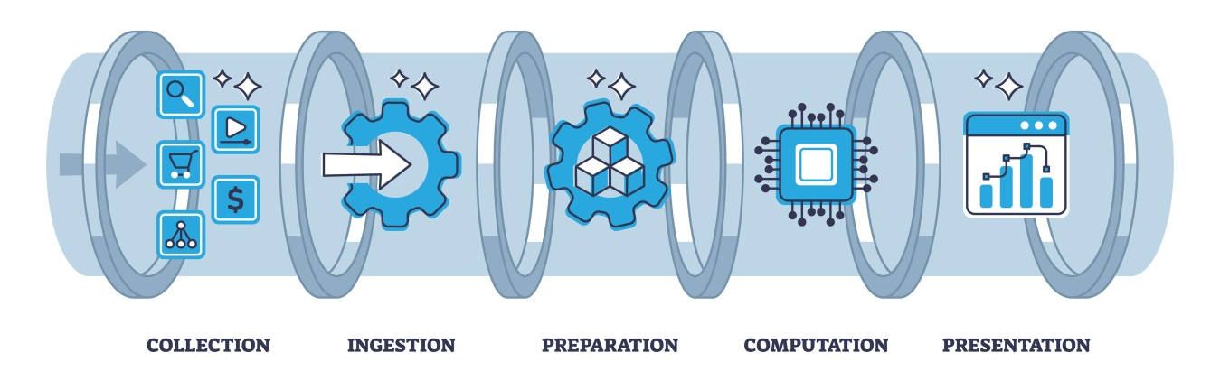
In this chapter, and over the next few, we’ll explore the core concepts of data and pipeline engineering, viewed from a systems perspective. This stage forms the structural backbone that supports the implementation of all subsequent stages in the MLOps lifecycle.
We’ll discuss:
- Data sources and formats
- ETL pipelines
- Practical Implementation
As always, every idea and notion will be backed by concrete examples, walkthroughs, and practical tips to help you master both the idea and the implementation.
Let’s begin!
Introduction: Understanding the data landscape
In machine learning operations (MLOps), success hinges not just on models but on the data pipelines that feed those models.
Production machine learning is a different beast entirely.
Here, the cleverest model architecture is worthless if it's fed unreliable data or if its predictions can't be reproduced (as we saw in earlier parts).
Hence, it is vital to have an understanding that, in the ML world, the raw material is data and the choices we make for data have profound downstream consequences on the performance, scalability, and reliability of our entire ML system.

Owing to the above fact, in an enterprise MLOps setting, engineers operate under a fundamental truth: models are often commodities, but the data and the pipelines that process it are the durable, defensible assets that drive business value.
Getting structured info from raw signals
Data in a production environment is not a clean, static CSV file. It is a dynamic, messy, and continuous flow of signals from a multitude of sources, each with its own characteristics and requirements.
Data sources
Production ML systems interact with data from several origins, like:
User input data
This is data explicitly provided by users, such as text in a search bar, uploaded images, or form submissions.
This data source is notoriously unreliable, since users are usually lazy, and if it's possible for a user to input unformatted and raw data, they will. Consequently, this data requires heavy-duty validation and robust error handling.
System-generated data (logs)

Applications and infrastructure generate a massive volume of logs.
These logs record significant events, system states (like memory usage), service calls, and model predictions.
While often noisy, logs are invaluable for debugging, monitoring system health, and, critically for us, providing visibility into our ML systems.
For many use cases, logs can be processed in batches (like daily or weekly), but for real-time monitoring and alerting, faster processing is required.
Internal databases
This is where enterprises typically derive most value from.
Databases that manage inventory, customer relationships (CRM), user accounts, and financial transactions are often the most valuable sources for feature engineering. This data is typically highly structured and follows a relational model.
For example, a recommendation model might process a user's query, but it must check an internal inventory database to ensure the recommended products are actually in stock before displaying them.
Third-party data
This is data acquired from external vendors. It can range from demographic information and social media activity to purchasing habits. While it can be powerful for bootstrapping models like recommender systems, its availability is increasingly constrained by privacy regulations.
Now that we broadly understand the sourcing of data for ML systems, let's also go ahead and understand some of the important data formats in the context of ML pipelines.
Data formats
The format you choose for storage is a critical architectural decision that directly impacts storage costs, access speed, and ease of use. The two most important dichotomies to understand are text versus binary and row-major versus column-major formats.
Text vs. Binary
Text formats like JSON and CSV are human-readable. You can open a JSON or CSV file in a text editor and immediately understand its contents.

This makes them excellent for debugging, configuration, and data interchange between systems. JSON, in particular, is ubiquitous due to its simplicity and flexibility, capable of representing both structured and unstructured data.
However, this readability comes at a cost: text files are verbose and consume significantly more storage space. Storing the number 1000000 as text requires 7 characters (and thus 7 bytes in ASCII), whereas storing it as a 32-bit integer in a binary format requires only 4 bytes.
Now, coming to binary formats like Parquet, these formats are not human-readable and are designed for machine consumption.
They are far more compact and efficient to process. A program must know the exact schema and layout of a binary file to interpret its bytes.

The space savings can be dramatic; for example, a 14 MB CSV file can be brought down to 6 MB when converted to the binary Parquet format. For large-scale analytical workloads, binary formats like Parquet are the industry standard.
Row-major vs. column-major
This distinction is perhaps the most critical for an ML engineer to grasp, as it directly relates to how we typically access data for training and analysis. It describes how data is laid out in memory.
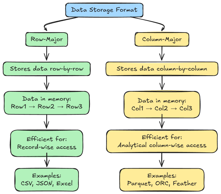
In row-major format (like CSV), consecutive elements of a row are stored next to each other. Think of it as reading a table line by line. This layout is optimized for write-heavy workloads where you are frequently adding new, complete records (rows).
It is also efficient if your primary access pattern is retrieving entire samples at once, for example, fetching all data for a specific user ID.
In column-major format (like Parquet), consecutive elements of a column are stored next to each other. This is optimized for analytical queries, which are common in machine learning. Consider the task of calculating the mean of a single feature across millions of samples.
In a column-major format, the system can read that one column as a single, contiguous block of memory, which is extremely efficient and cache-friendly. In a row-major format, it would have to jump around in memory, reading a small piece of data from each row, which is significantly slower.
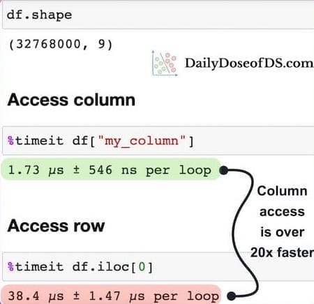
The performance implications are not subtle. The popular pandas library, for instance, is built around the column-major DataFrame.
A common scenario is to iterate over a DataFrame row by row. This can be orders of magnitude slower than iterating column by column.
This snippet reveals that iterating a DataFrame of 32M+ rows by column takes just under 2 microseconds, while iterating the same DataFrame by row takes 38 microseconds, which is a ~20x difference.
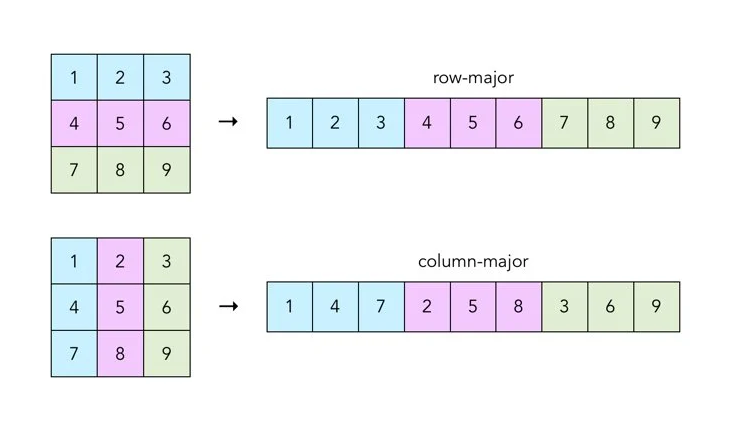
This happens because, as mentioned above, a Pandas DataFrame is a column-major data structure, which means that consecutive elements in a column are stored next to each other in memory, as depicted below:
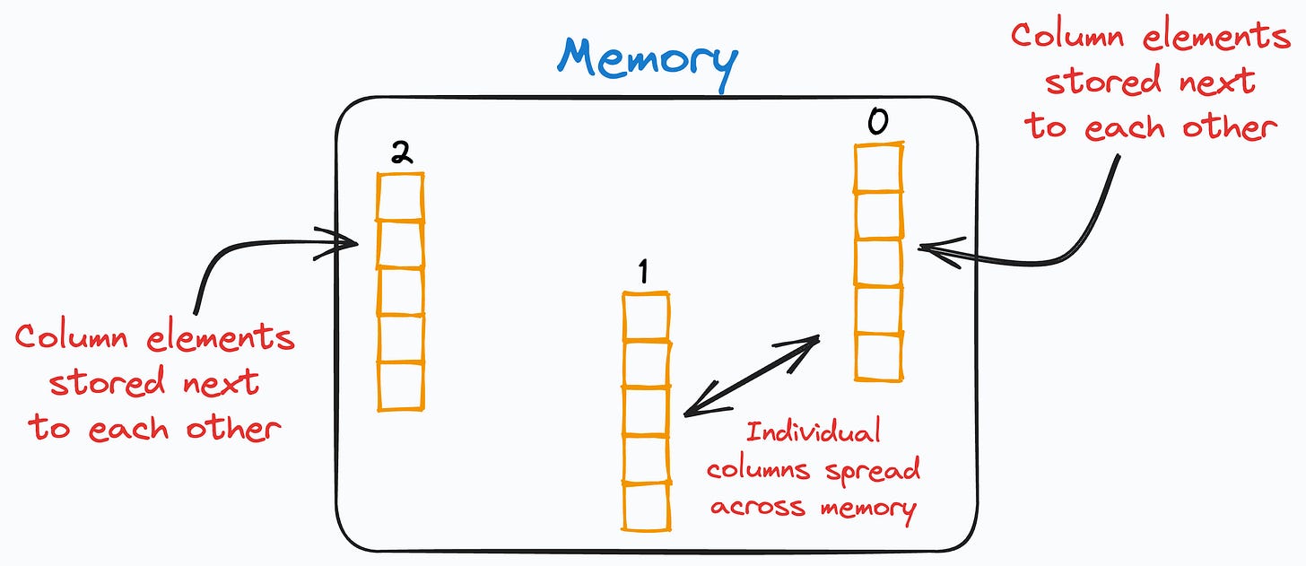
The individual columns may be spread across different locations in memory. However, the elements of each column are ALWAYS together.
As processors are much more efficient with contiguous blocks of memory, retrieving a column is much faster than fetching a row.
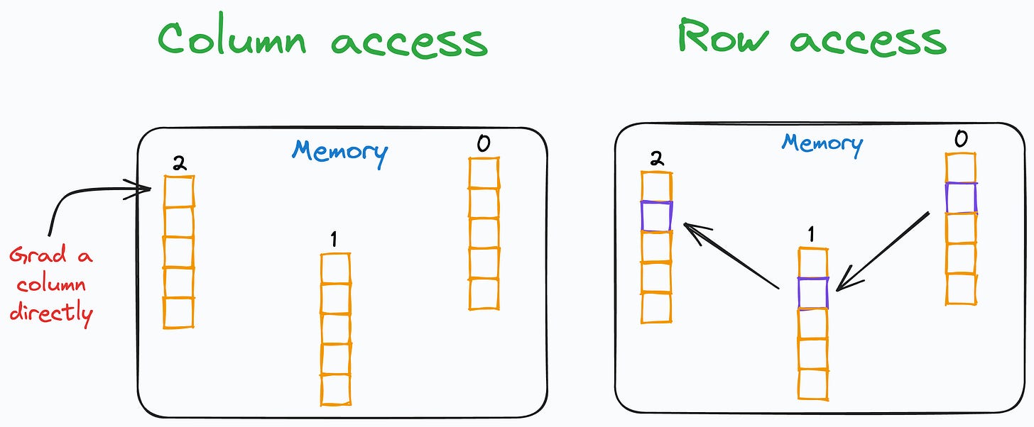
In other words, when iterating, each row is retrieved by accessing non-contiguous blocks of memory. The processor must continually move from one memory location to another to grab all row elements.
As a result, the run-time increases drastically.
This isn't a flaw in pandas; it's a direct consequence of its underlying column-major data model.
With an understanding of data sourcing and formats in place, let's now explore one of the core concepts of data engineering: ETL pipelines.
Data engineering foundations: ETL
Before building pipelines, we need a solid grasp of data engineering fundamentals in an ML context. Hence, let's see how raw data is extracted, processed, and organized for machine learning workflows.
ETL in ML workflows
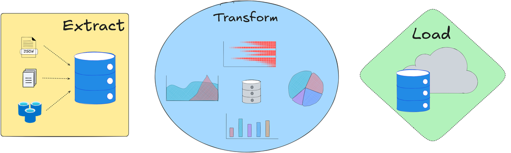
ETL stands for Extract, Transform, Load. It describes the pipeline of getting data from sources, processing it into a usable form, and loading it into a storage or system for use. ETL is often the first stage of preparing data for model training or inference.
Let's briefly discuss each stage theoretically:
Extract
Pull data from various sources (databases, APIs, files, etc.). In ML workflows, sources could include application databases, logs, third-party datasets, user-provided data, etc.
Extraction involves reading this data and often validating it (e.g., checking for malformed records). You should reject or quarantine data that doesn’t meet expectations as early as possible to save trouble downstream.
For example, if extracting data from a user input feed, you might filter out records with missing required fields and log or notify the source about the bad data. Early validation during extraction can prevent propagating errors.
Transform

This is the core processing step where data is cleaned and converted into the desired format.
This can include merging multiple sources, handling missing values, standardizing formats (e.g., making categorical labels consistent across sources), deduplicating records, aggregating or summarizing data, deriving new features, and more.
In ML terms, transformation includes feature engineering, that is, turning raw data into features that models can consume. For instance, transforming raw timestamps into features like day-of-week or time-since-last-event, encoding categorical variables as one-hot vectors, and normalizing numeric fields.
The transform phase is actually the "hefty" part of the process where most data wrangling happens.
Load

Finally, load the transformed data into a target destination. The target might be a data warehouse, a relational database, a distributed storage, cloud storage, or an analytical database, depending on the use case.
In ML pipelines, the “load” step could mean writing out a cleaned dataset for training (e.g., as a CSV/Parquet file, or to a data warehouse table), or loading features into a feature store or into production databases for serving.
Key considerations are how often to load (batch schedule or streaming) and in what format. For example, you might load aggregated features daily into a warehouse table that the model training job will read.
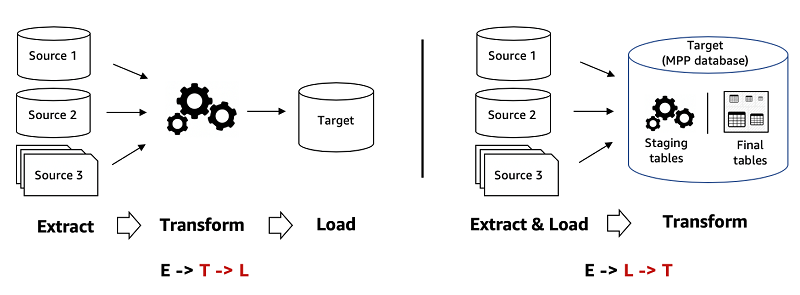
ETL vs. ELT
You might encounter the term ELT (Extract, Load, Transform). This is a variant where raw data is first loaded into a storage (often a data lake) before transformation.
ELT has become popular with the rise of inexpensive storage and scalable compute. Organizations dump all their raw data into a data lake (like an S3 bucket or HDFS) immediately, and transform it later when needed.
The advantage is quick ingestion (since minimal processing is done upfront) and flexibility to redefine transformations later.
However, the downside is that if you store everything raw, you later face the cost and complexity of sifting through a “data swamp” to find what you need; as data volume grows, scanning a massive lake for each query can be inefficient.
Hence, the key is to balance fast data acquisition (ELT style) with upfront processing (ETL style) to keep data usable.
In ML, a common pattern is to do some light cleaning upon extraction (to avoid garbage data accumulation), load into a lake/warehouse, then do heavier feature engineering transformations in later pipeline stages before model training.
Example: ETL for ML
Imagine an e-commerce company building a recommendation model. The ETL pipeline might extract data from production databases (orders, user info, product catalog), then transform it by joining tables, cleaning out inactive users or test orders, aggregating purchase history per user, and encoding product categories.
The transformed feature set (say, a table of user features and labels for recommendation) is then loaded into a data warehouse table or saved as a file. The ML training job later simply reads this prepared data.
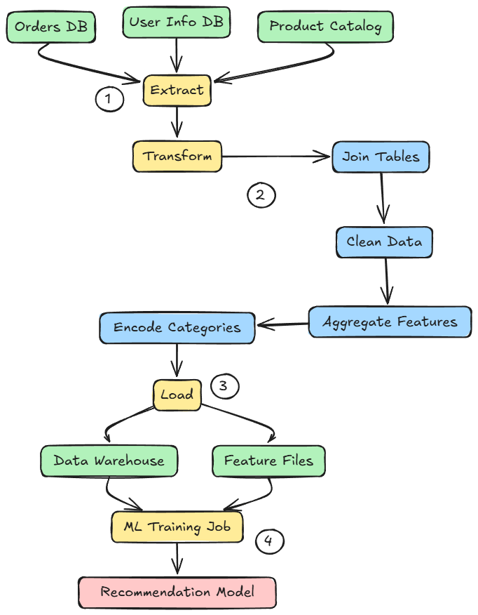
Hence, this is one of the ways an ETL pipeline can be designed and implemented.
If the company instead did ELT, they would dump all raw logs and databases into a data lake, and the ML pipeline would have to transform raw data on the fly each time, which is more flexible, but possibly slower. Often, a hybrid is used: some ETL to create intermediate features, then maybe ELT of those into a warehouse and further transformations.
Note on streaming
ETL traditionally implies batch processing (periodic loads). If you have streaming data (real-time) feeding into an online model, similar principles apply, but with streaming tools (like Kafka for extraction, real-time transforms, etc.).
We’ll touch on streaming in the context of feature stores and orchestration in a future chapter, but the foundational idea of “get data → process → use data” remains, just with low latency.
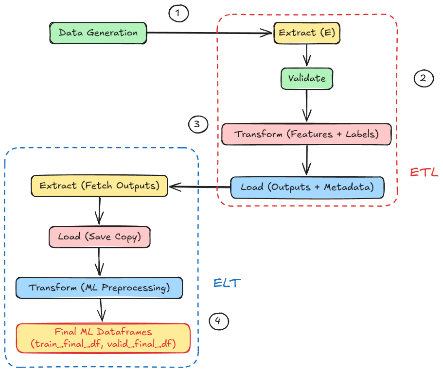
Hands-on: Building data pipelines
In this section, we’ll simulate a basic machine learning data pipeline using Pandas, NumPy, and Scikit-learn.
Objectives:
- Generate synthetic data to simulate data collection from multiple sources.
- Explore different file formats commonly used in data pipelines.
- Implement a hybrid ETL/ELT approach, demonstrating practical data transformation workflows.
- Obtain the final processed dataframes.
Through this hands-on simulation, our goal is to develop a foundational understanding of how data pipelines function in ML-centric setups and how the practical behavior aligns with theory.
Project setup
This project's code is meant to be run using Google Colab. We recommend uploading the .ipynb notebook in Colab, and running it from there.
Download the notebook here: