Monitoring and Observability: Core Fundamentals
MLOps Part 16: A comprehensive overview of drift detection using statistical techniques, and how logging and observability keep ML systems healthy.
Recap
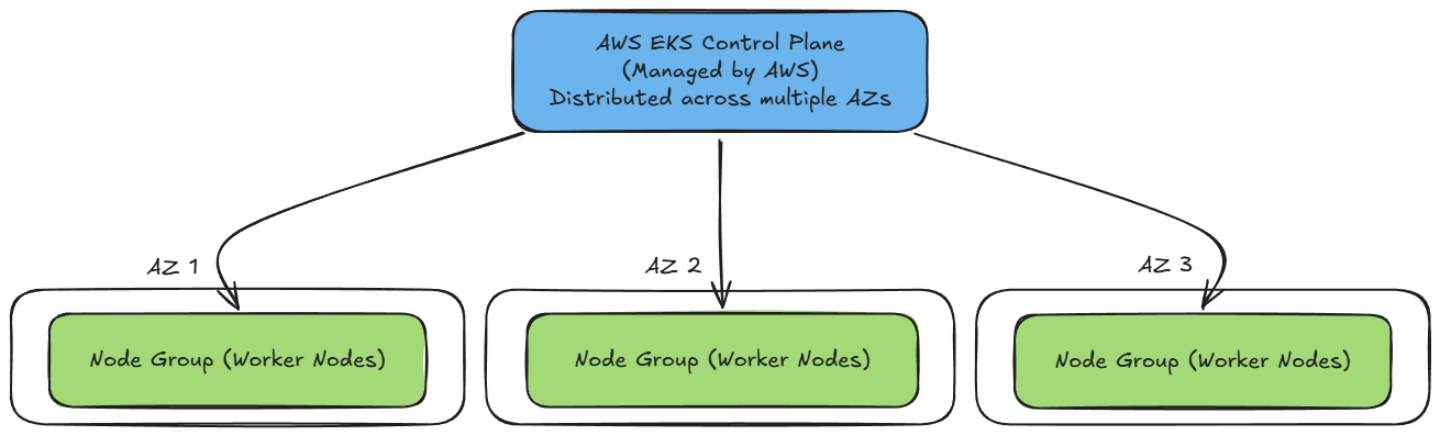
In Part 15 of this MLOps and LLMOps crash course, we explored AWS and its services, particularly AWS EKS.

We began by exploring the fundamentals and gaining an overview of AWS EKS. This included learning about the EKS lifecycle and various stages that fall into it.
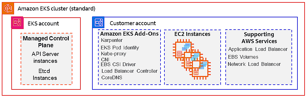
After that, we explored the integration of EKS into the broader AWS ecosystem, understanding IAM, networking, storage, security, and monitoring.
Next, we did a brief discussion on the design and operational considerations for AWS EKS, understanding cluster topology, networking, storage, cost, and observability.
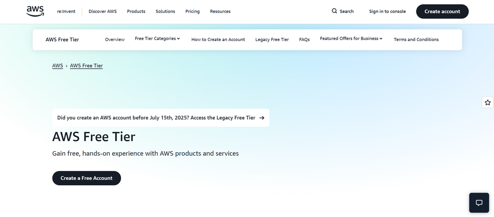
Moving ahead, we saw how to set up a personal AWS Free Tier account for our learning and experimentation activities.
Finally, we went hands-on with setting up one EKS cluster and deploying our Kubernetes workload on it.
If you haven’t explored Part 15 yet, we strongly recommend going through it first, since it sets the foundations and flow for what's about to come.
Read it here:

In this chapter, we’ll continue our discussion of the deployment and monitoring phase, shifting our focus from deployment aspects to monitoring, and understanding the fundamentals of monitoring and observability.
As always, every notion will be explained through clear examples and walkthroughs to develop a solid understanding.
Let’s begin!
Introduction
Deploying a machine learning model into production is often celebrated as a major milestone in the development lifecycle.
However, as we have seen earlier, this deployment marks not the end of the journey, but the beginning of a new and complex phase often referred to as the “day two” problem, known as monitoring and observability.
Once a model is live, it begins interacting with real-world data and users, i.e., environments that are dynamic, evolving, and frequently unpredictable. In this setting, the model’s performance can no longer be taken for granted; maintaining its accuracy, reliability, and business value requires continuous attention.
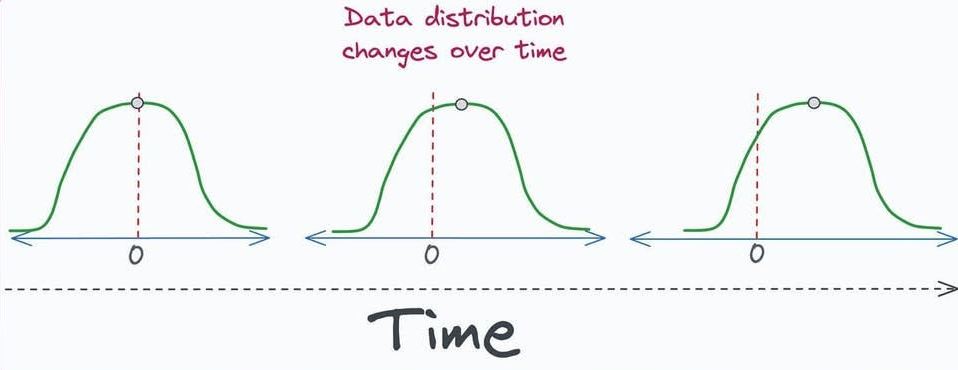
In production, numerous factors can cause a well-trained model to degrade over time. Data distributions may shift due to seasonal trends, new customer behaviors, or changes in market conditions.
Upstream data pipelines can fail, introducing missing or corrupted features. Even small alterations in external systems or user interfaces can lead to significant changes in how data is generated and consumed.
Unlike the static conditions of a test environment, the real-world ecosystem is fluid and interconnected, making it prone to hidden issues that can silently erode model performance.
This phenomenon highlights the importance of robust monitoring. The systematic observation, measurement, and maintenance of machine learning models after deployment allows teams to detect performance degradation and operational anomalies early, enabling timely interventions before these issues affect end users or business outcomes.
Beyond tracking metrics, MLOps monitoring involves a proactive culture of accountability and continuous improvement. It ensures that models remain trustworthy, interpretable, and aligned with evolving real-world conditions.
In essence, while model deployment marks the beginning of value creation, it is ongoing monitoring that sustains and safeguards that value over time.
This initial chapter on model monitoring will explain the fundamentals of monitoring and observability so that you can build reliable ML systems.
Why do models degrade?
A traditional software bug is often loud and obvious: a server crashes, a webpage returns a 404 error, or an application throws an exception. The failures in machine learning systems, however, are frequently silent.
The API continues to return predictions with low latency and 200 OK status codes, yet the predictions might themselves become progressively less accurate and less useful.
This silent degradation can go unnoticed for weeks or months, slowly eroding business value and user trust. To build a resilient MLOps practice, it is essential to first understand the taxonomy of these failures, providing a mental model to diagnose problems when they inevitably arise.
Software vs. ML-specific issues
Failures in a production ML system can be broadly categorized into two groups: traditional software system failures and ML-specific failures:
Software system failures
These are issues that can affect any complex software system, not just those involving machine learning. These include:
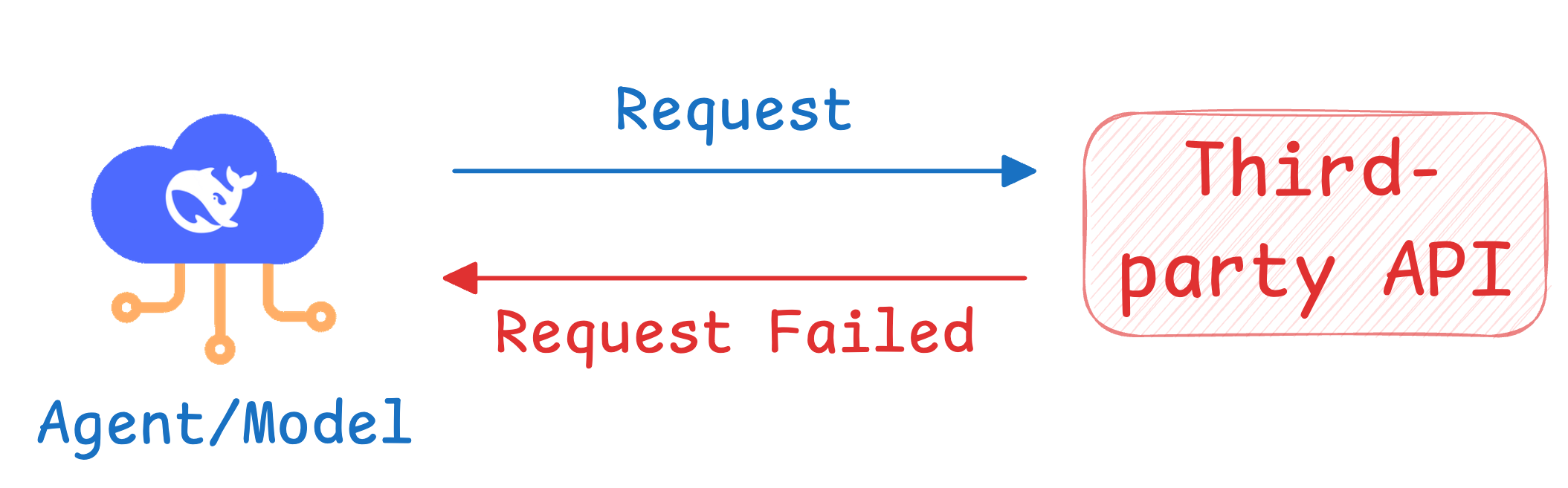
- Dependency failures: An upstream service or a third-party software package that the system relies on breaks or changes its API.
- Deployment errors: The wrong model binary is accidentally deployed, or the service lacks the correct permissions to access necessary resources.
- Hardware failures: CPUs overheat, GPUs fail, or the network infrastructure goes down.
- Bugs in distributed systems: Errors in the workflow scheduler, data pipeline joins, or other components of the surrounding infrastructure.
Addressing these issues requires strong, traditional software engineering and DevOps skills. The prevalence of these failures underscores the fact that MLOps is, to a large extent, an engineering discipline.
ML-specific failures
These are the subtle failures that are unique to systems that learn from data.
They do not typically cause crashes but result in a degradation of the model's predictive performance. These failures often occur silently because the system continues to operate from a technical standpoint, even as its outputs become nonsensical.
The upcoming sections will explore the most common types of these failures in detail.
Understanding model degradation
As we already understand, while traditional software systems typically fail in clear and predictable ways, machine learning models often degrade subtly as their environment evolves.
This degradation stems from shifts in data, changes in user behavior, or gradual mismatches between the model’s assumptions and real-world conditions.
To effectively monitor and maintain model performance, it’s crucial to understand the different forms these issues can take.
Data and concept drift
The most fundamental and pervasive ML-specific failure is caused by distribution shifts. This occurs when the statistical properties a model encounters in production differ from what it was trained on.
The core assumption of supervised learning, that the training and production data are drawn from the same underlying distribution, is almost always violated in the real world.
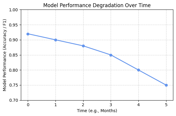
Hence, it is a common phenomenon that once an ML model is deployed, its performance can deteriorate over time due to drift.
Data drift
Data drift usually refers to changes in the input data distribution, which could be covariate shift (features’ distributions shift).
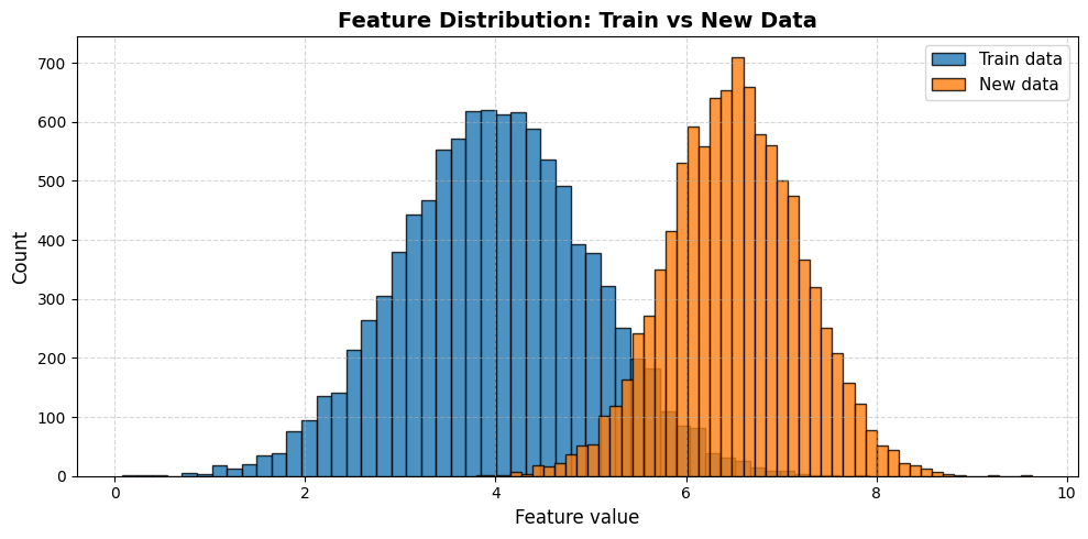
For example, if a model was trained on transaction data from last year, but this year a new demographic of users is using the platform, and hence feature distributions might shift.
Another example could be that a marketing change leads to a younger audience, so the age feature distribution changes, potentially degrading a model's performance.
Now, based on what we understand, we might be tempted to think that a data drift that happens should necessarily trigger a set of actions immediately, but it is important to understand that not all data drift is catastrophic.
Sometimes models generalize fine to the new distribution (e.g., a slight shift in age might not matter if the model is robust). But significant drift can break the model’s assumptions.
Thus, detecting data drift is about monitoring feature stats: mean, standard deviation, minimum/maximum, distributions, correlations, etc., and seeing if they deviate from the training stats beyond a certain threshold.
Concept drift
This indicates that the world changed such that even if the input distribution is the same, the output (target) mapping has changed.
To state technically, concept drift refers to changes in the relationship/mapping between inputs and outputs (the underlying concept that the model is trying to predict).
For instance, in the two plots below, both features span the same range of values before (feature 1 ranges from [0, 10] and feature 2 ranges from [2, 10]) and after drift (feature 1 ranges from [0, 10] and feature 2 ranges from [2, 10]), but the mapping has changed:
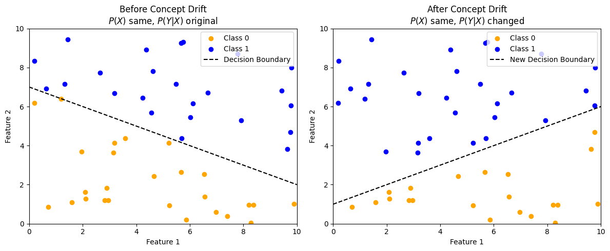
A classic example can be a model predicting customer churn. Before the pandemic, the model might have learned that users who logged in less than twice a week and didn’t engage with premium features were likely to churn.
After the pandemic, however, usage patterns shifted, and even highly active users began canceling subscriptions due to budget cuts or changes in personal priorities.
As another example, consider a credit card fraud detection model.
Before, fraudulent transactions might typically involve small purchases from foreign IPs made within minutes of each other, which became a clear red flag.
Over time, fraudsters adapt. They start mimicking genuine behavior by making larger, domestic transactions spread out over several hours or by routing through local proxies to appear legitimate.
The model’s input features, like the transaction amount, location, and timing, still fall within familiar ranges, but the relationships between them and the likelihood of fraud have changed. The model’s old concept of “fraudulent” is now outdated, leading to concept drift.
Concept drift usually requires retraining on more recent data to catch the new relationships. Unlike data drift, which sometimes the model can handle if within its learned range, concept drift almost always implies the model is now suboptimal and needs an update.
Training-serving skew
Training-serving skew is a particularly common and frustrating issue that is not caused by external changes in the world, but rather by internal discrepancies in the ML pipeline itself.
It occurs when the feature data used during model training is different from the feature data used during online inference. This is often a self-inflicted wound caused by process or implementation errors.
Hence, we need to understand that this is more about the process, i.e., if the data the model gets in production is processed differently from training data, it can cause performance issues.

For example, if a feature was normalized in training, but in production, the normalization isn’t applied correctly, the model input is skewed.
This is why ensuring the feature engineering code is consistent (or using a feature store for both train and serve) is important.
Monitoring can catch some of this, for example, if a feature’s mean in production is way off from training, maybe it’s a bug.
Let's explicitly mention some of the common causes that lead to this, so you can be mindful of them:
- Separate codebases: The feature engineering logic for training is often written in a data science-friendly environment (e.g., Spark/Pandas) that processes data in batches. The logic for serving, however, might be rewritten in a low-latency language (e.g., C++). Any subtle difference in the implementation of a feature between these two codebases might introduce skew.
- Data pipeline bugs: A bug in the production data pipeline can cause features to be generated incorrectly. For example, a data source might become unavailable, causing a feature to be filled with NaNs or default values in production, while the training data was clean.
- Time window discrepancies: A feature might be defined as "the number of user clicks in the last 30 days." If the training pipeline correctly uses a 30-day window but a bug in the serving pipeline causes it to only use a 15-day window, this might introduce significant skew.
Mitigating training-serving skew is a primary motivation for adopting a feature store, which provides a centralized repository for feature definitions and logic, ensuring that the same transformations are applied in both training and serving environments.
We already covered feature stores in an earlier chapter of this series. Check it out below:
Outliers
An outlier is an individual data point very different from the training data. Monitoring for outliers can be as simple as seeing if feature values fall outside expected ranges (e.g., negative values where none existed, or extremely large values).
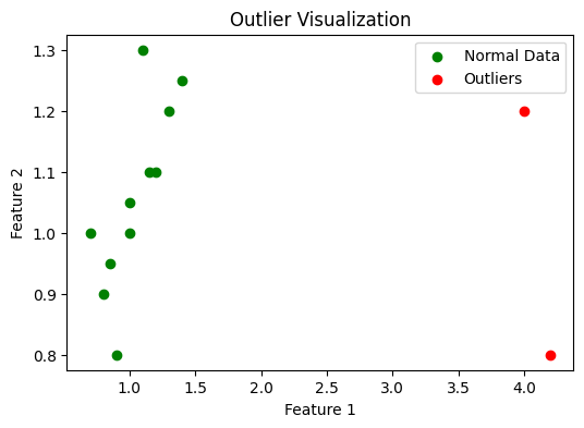
In fraud detection, if a model was never trained on transactions above \$1 million and one day it sees a \$15 million transaction, that’s an outlier. The model’s prediction on it will likely be unreliable.
Detecting such events (and perhaps routing them for special handling) is important. Sometimes outliers can be the first hint of drift (e.g., a few outlier instances appear before the whole distribution shifts).
Now that we understand the key reasons for the degradation of model performance, let's go ahead and learn about a few detection techniques, especially for drifts.
Techniques to detect drift
There are several robust statistical and algorithmic methods to detect both data drift (changes in feature distributions) and concept drift (changes in the relationship between features and labels).
Common statistical approaches include the Kullback-Leibler (KL) divergence, Population Stability Index (PSI), and the Kolmogorov-Smirnov (KS) test, while more adaptive methods like ADWIN (Adaptive Windowing) are often used for continuous monitoring.